Hamiltonian System and Classical Mechanics

Adv. Theor. Appl. Mech., Vol. 1, 2008, no. 5, 217 – 224

Hamiltonian System and Classical Mechanics V.G. Gupta and Patanjali Sharma Department of Mathematics, University of Rajasthan, Jaipur-302 004, India [email protected] and [email protected]

Abstract In this paper the formalism of Hamiltonian system ( X , ω , H ) on the symplectic manifold due to Reeb [2] given in Abraham and Marsden [4] and Arnold[5] is used to derive the equations of motion (1) for a particle in a line with a bona fide solution (2) for a free particle in three-space with Hamiltonian and non-Hamiltonian flow, it is also shown that the non-Hamiltonian flow can be converted into a Hamiltonian flow by changing symplectic form and the phase space. Keywords: Symplectic Hamiltonian Flow

Manifold,

Hamiltonian

System,

Phase-Space,

(1.1) Introduction The use of differential form in mechanics and its eventual formulation in terms of symplectic manifolds has been slowly evolving since Cartan [1]. In a closed system the energy is constant as the physical system moves in time. For any given physical system, each known conserved quantity provides an equation that can be very useful in the analysis of the system. But energy is more than a conserved quantity, it determine the equation of motion. All conceivable information about the system is hidden in the energy formula. Unpacking this information is a mathematical problem. In this paper we will use the Hamiltonian system to derive the equations of motion in classical mechanics from the energy function and the kinetics of phase space. In other words, we will show how a real-valued function on a symplectic manifold determines a vector field. The energy function is known as Hamiltonian function and is denoted by H. The corresponding vector field on phase space is called a Hamiltonian vector field and is denoted by X H .This vector field corresponds naturally to a system of first-order differential equations on phase space, which in physical system is equivalent to Newton’s second law (Force = mass × acceleration). The solution of the

218

V.G. Gupta and Patanjali Sharma

differential equations is the Hamiltonian flow. Physically the Hamiltonian flow gives us possible physical motions.

(1.2) Hamiltonian System A general Hamiltonian system consists of a manifold X , possibly infinite dimensional together with a (weakly) non-degenerate closed two-form ω on X (i.e. ω is an alternating bilinear form on each tangent space Tx X of X , d ω = 0 , and for x ∈ X , ω x (u , v) = 0 for all u ∈ Tx X implies v = 0 ) and a Hamiltonian function H : X → R .Then X , H, ω determine in nice cases, a vector field X H called the Hamiltonian vector field. Let X be a Banach manifold and let X o be a manifold domain of X . Let H be a ∞

C function on X o into R called the Hamiltonian or energy function, then for each x ∈ X o , d x H : Tx X o → R is a continuous linear function. Let ω be a C ∞ covariant

tensor field of order two on a C ∞ manifold domain X o such that for each x ∈ X o ,

ω x : Tx X o × Tx X o → R is non-degenerate, for each x ∈ X o , let λx : Tx X o → Tx* X o be the isomorphism induced by ωx and is defined by λ (u ).(v) = ωx (u , v) ∀ x ∈ X o ; u, v ∈ Tx X o * Denote λ :TX o → T X o where λx = λ T X for each x ∈ X o , this λ is a vector bundle x

o

isomorphism of TX o onto T * X o . Then ω and H induces a C ∞ vector field X H = λ −1 o dH on X o , determined by the condition C X H ω = dH

(1.2.1)

(1.3) Flow Let X be a smooth manifold. A smooth function F : R × X → X is called a flow for the vector field v if F⋅ x : R → X is an integral solution for v i.e. d F⋅ x (t ) = v o F⋅ x (t ) dt d or F (t , x) = v o F (t , x) dt and F⋅ x (0) = F (0, x) = x ∀ t ∈ R, x ∈ X

(1.4) Hamiltonian Flow

Hamiltonian system and classical mechanics

219

Let ( X , H , ω ) be a Hamiltonian system. A flow F is called a Hamiltonian flow if it preserves the symplectic form and Hamiltonian function (i.e. Ft ∗ω = ω and Ft ∗ H = H for t ∈ R ) see Abraham & Marsden[4]. Here, it should be noted that the symplectic form plays a crucial role i.e. without changing the Hamiltonian function but changing the symplectic form we can get different flows i.e. vector fields.

(2.1) The motion of a particle on a line in a plane Here we consider the example of physical system whose phase space is the simplest non-trivial symplectic manifold, the two-dimensional plane X = R 2 = {(r , p) : r ∈ R, p ∈ R} with the area two-form ω = dr ∧ dp . Consider a particle of mass m moving on a line, subject to no forces, such a particle is called a free particle, any free particle travels with constant speed. Thus the Hamiltonian 1 2 function for such a particle is H = p . The equation C X H ω = dH gives the 2m X H for any r ∈ R , v ∈ Tx R and taking Hamiltonian vector field ∂ ∂ ∂ ∂ as arbitrary vector field, we find X H = xr + xp and v = vr + vp ∂r ∂p ∂r ∂p ∂ ∂ ∂ ∂ p ∂ ∂ , vr + xp + v p ) = ( dp)(vr + vp ) ∂r ∂p ∂r ∂p m ∂r ∂p p xr v p − x p vr = v p m p xr = and x p = 0 . m

(dr ∧ dp)( xr or ⇒ Thus, we have

p ∂ m ∂r since r and p are functions of time t(along a particular trajectory ), taking the dr ∂ dp ∂ as time derivative along trajectories on the vector field X H = . + . dt ∂r dt ∂p plane, we have p ∂ dr ∂ dp ∂ = . + . m ∂r dt ∂r dt ∂p ∂ ∂ Since, and are linearly independent, we have ∂r ∂p XH =

220

V.G. Gupta and Patanjali Sharma

dp p dr =0. = and dt m dt

(2.1.1)

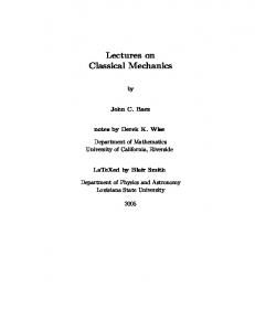
which shows that a free particle travels with constant momentum along the line. d 2r This is equivalent to 2 = 0 , the equation of motion for the free particle. dt Since the Hamiltonian flow preserves the Hamiltonian and the symplectic form we can use this conservation of the Hamiltonian by the Hamiltonian flow to draw useful pictures, because it implies that the orbits of the system must lie inside level sets of H . (an orbit a set of all points in phase space that the system passes through , during on particular motion. In other words it is the set of all points on one particular trajectory). The beautiful features of Hamiltonian systems is that we can get information about orbits of the differential equations of motion by solving the algebraic equation H = constant, which is easy to solve. For example, if we consider the motion of a free particle on the line then the conservation of the Hamiltonian by the Hamiltonian flow tells us that orbits must lie inside sets of the form p2 H= = constant. Since the motion is continuous, it follows that each orbit is 2m contained in a line p = constant (see figure 1). Here it should be noted that not every orbit is an entire line. The r-axis ( p = 0) is made up of single-point orbit representing motionless particles. All other orbits are entire lines representing particles moving at constant velocities. p

r

Figure 1 : phase space of the particle on the line with level sets of the force free Hamiltonian.

Hamiltonian system and classical mechanics

221

If we desire to find bonafide solutions to our differential equation, i.e., we desire to know not only the orbit of a trajectory but the trajectory itself (i.e., the position as a function of time). We have to solve one differential equation than solving the original dp dr p system of differential equations ( = and = 0 ). dt dt m Let

⇒

p2 H0 = 2m p = ± 2m H 0

2H 0 dr (2.1.2) =± dt m We take plus sign if the orbit lies on a line above the r-axis, otherwise we take the minus sign. Now we can easily integrate the above equation (2.1.2) to get 2H 0 r (t ) = ± t + r (0) m initially when t = 0 , p (t ) = p (0) , so t r (t ) = p(0) + r (0) m for any fixed t , the flow map ft : R 2 → R 2 defined by

or

p ⎞ ⎛ ⎛ r ⎞ ⎜r + t⎟ m ⎜ ⎟a ⎜ ⎝ p ⎠ ⎜ p ⎟⎟ ⎝ ⎠ preserves symplectic form ω = dr ∧ dp . For, ft ∗ (dr ∧ dp ) = f t ∗ (dr ) ∧ f t ∗ (dp ) t = (dr + dp) ∧ dp m = dr ∧ dp = ω .

(2.2) Motion of a free particle in Three-Space Consider the motion of a free particle in three space. Let r = (r1 , r2 , r3 ) be the position vector of the particle and p = ( p1 , p2 , p3 ) be the corresponding momentum of the particle. Then the phase space of the particle is the manifold X = {(r1 , r2 , r3 , p1 , p2 , p3 ): r1 , r2 , r3 , p1 , p2 , p3 ∈ R } with the symplectic form ω = dr1 ∧ dp1 + dr2 ∧ dp2 + dr3 ∧ dp3 . The Hamiltonian function of the system is

222

V.G. Gupta and Patanjali Sharma

1 ( p12 + p22 + p32 ) . Then ( X , ω , H ) determine vector field X H by the 2m condition (1.2.1). i =3 ∂ ∂ ∂ ∂ ∂ ∂ ∂ ∂ v + a2 + a3 + b1 + b2 + b3 + bi′ and = ∑ ai′ Let X H = a1 ∂ri ∂pi ∂r1 ∂r2 ∂r3 ∂p1 ∂p2 ∂p3 i =1 be arbitrary vector fields, then using (1.2.1), we have ω ( X H , v) = dH (v) H=

or

i =3

i =3

i =1

i =1

( ∑ dri ∧ dpi ) ( ∑ ai

∂ ∂ i =3 ′ ∂ ∂ + bi + bi′ , ∑ ai ) ∂ri ∂pi i =1 ∂ri ∂pi

=[ i =3

or

1

i =3 1 i =3 ∂ ∂ (∑ pi dpi ) ](∑ ai′ + bi′ ) ∂ri ∂pi m i =1 i =1 i =3

∑ (a b ′ − a ′b ) = m (∑ p b ′ ) i =1

i i

i

i

i =1

i

i

This gives, pi and bi = 0 , i=1,2,3. m Thus the vector field is given by p ∂ p ∂ p2 ∂ XH = 1 + + 3 m ∂r1 m ∂r2 m ∂r3 Taking the vector field, dp ∂ dr ∂ dr2 ∂ dr3 ∂ dp1 ∂ dp2 ∂ XH = 1 + + + + + 3 dt ∂r1 dt ∂r2 dt ∂r3 dt ∂p1 dt ∂p2 dt ∂p3 as time derivative along trajectories, we have dpi p1 dr1 p2 dr2 p3 dr3 = = , , = and =0 , i = 1,2,3. m dt m dt m dt dt This gives, d2 m 2 (r) = 0 dt This is the required equation of motion of the free particle in three- space. It is evident from above that for any fixed time t , the map f t : R 3 × ( R 3 )∗ → R 3 × ( R 3 )∗ ai =

p ⎞ ⎛ ⎛ r ⎞ ⎜r + t ⎟ defined by m ⎜ ⎟a ⎜ ⎝ p ⎠ ⎜ p ⎟⎟ ⎝ ⎠ is a Hamiltonian flow as it preserves ω = dr1 ∧ dp1 + dr2 ∧ dp2 + dr3 ∧ dp3 and the 1 ( p12 + p22 + p32 ) , for H= 2m

(2.2.1)

(2.2.2)

(2.2.3)

the symplectic form Hamiltonian function

Hamiltonian system and classical mechanics

223

i =3

ft ∗ ω = ft ∗ (∑ dri ∧ dpi ) i =1

i =3

= ∑ ( ft ∗ dri ∧ ft ∗dpi ) i =1 i =3

= ∑ (dri + i =1 i =3

t dpi ) ∧ dpi m

= ∑ (dri ∧ dpi ) = ω i =1

∗

and ft H = H , as ft changes only the values of r, while H depends only on p. So ft preserves the Hamiltonian. Now to show that every flow is not a Hamiltonian flow. Consider an example of the motion of a free particle in space having the flow, g t : R 3 × ( R 3 )∗ → R 3 × ( R 3 ) ∗ ⎛ r ⎞ ⎛ r et ⎞ defined by (2.2.4) ⎜ ⎟a ⎜ t ⎟ ⎝p⎠ ⎝ pe ⎠ for any t ∈ R , then gt∗ω = e2tω shows that the flow gt does not preserves the symplectic form. Hence it is not the Hamiltonian flow of a Hamiltonian system with the canonical symplectic form on R 6 . i =3 1 (dri ∧ dpi ) then the Now if we define the symplectic form on R 6 ~ {0} as ω = ∑ i =1 ri pi flow gt defined by (2.2.4) preserves ω , for i =3

gt∗ω = gt∗ ( ∑ i =1

i =3

= ∑ gt∗ ( i =1

i =3

=∑ i =1

i =3

=∑ i =1

i =3

=∑ i =1

1 (dri ∧ dpi ) ) ri pi

1 dri ∧ dpi ) ri pi

1 ( d (ri et ) ∧ d ( pi et ) ) t (ri e pi e ) t

1 e 2t (dri ∧ dpi ) 2t (ri pi e ) 1 (dri ∧ dpi ) (ri pi )

=ω. order to find the Hamiltonian function for this system, let i =3 ∂ ∂ ∂ ∂ ∂ ∂ ∂ ∂ X H = r1 + r2 + r3 + p1 + p2 + p3 and v = ∑ ai′ be an + bi′ ∂ri ∂pi ∂r1 ∂r2 ∂r3 ∂p1 ∂p2 ∂p3 i =1 arbitrary vector field then using (1.2.1), we have ω ( X H , v) = dH (v)

In

224

V.G. Gupta and Patanjali Sharma i =3

or

∑( i =1

i =3 1 ∂ ∂ i =3 ′ ∂ ∂ , ∑ ai ) = dH (v) dri ∧ dpi ) ( ∑ ri + pi + bi′ ri pi ∂ri ∂pi i =1 ∂ri ∂pi i =1

i =3

or

∑( i =1

1 ′ ′ (rb i i − ai pi ) ) = ( ri pi

i =3 i =3 ∂H ∂H ∂ ∂ ) ( ) dr dp ai′ + + bi′ ∑ ∑ ∑ i i ∂ri ∂pi i =1 ∂ri i =1 ∂pi i =1 i =3

This gives,

∂H 1 ∂H 1 , =− = ri ∂ri ∂pi pi which on integration yields, ⎛pp p ⎞ H = log ⎜ 1 2 3 ⎟ + c ⎝ r1r2 r3 ⎠ Now, ⎛pp p ⎞ gt∗ H = g t∗ ( log ⎜ 1 2 3 ⎟ + c ) ⎝ r1r2 r3 ⎠

(2.2.5)

⎛ ( p et )( p et )( p3et ) ⎞ = log ⎜ 1 t 2 t ⎟+c t ⎝ (r1e )(r2 e )(r3e ) ⎠ =H Hence gt also preserves H . Thus gt defined by (2.2.4) is a Hamiltonian flow for i =3

the Hamiltonian system ( M , ω , H ) , where M = R 6 − {0} , ω = ∑ i =1

1 (dri ∧ dpi ) and ri pi

H is given by (2.2.5).

References [1] E. Cartan, Lecons sur les invariants integraux, Hermann, Paris, 1922. [2] G. Reeb, Varietes symplectiques, Varietes Presque-Compleses et systemes dynamiques, C.R. Acad. Sci. Paris 235(1952), 776-778. [3] G.F. Simmons, Differential Equations with applications and historical notes, Second Edition, McGraw Hill, Inc., New York 1991. [4] R. Abraham and J. Marsden, Foundations of mechanics, Second Edition, Addison-Wesley, Reading, MA, 1978. [5] V.I. Arnold, Mathematical methods of Classical Mechanics, Second Edition, Springer-Verlag, New York, 1989. Received: April 22, 2008