Hamiltonian Vector Field for the Lorenz Invariant Set Andrzej Lozowski, Rafal Komendarczyk and Jacek M. Zurada Department of Electrical Engineering, University of Louisville, Louisville, Kentucky 40292 e-mail:
[email protected],
[email protected] Abstract The existence of a Hamiltonian vector field in which trajectories of the invariant set of a dissipative hyperbolic chaotic system are embedded will be proved (see notation below). Evidence of this with an example concerning the Lorenz system will be provided. Also, a constructive method of designing a Hamiltonian for the Lorenz attractor with a universal approximator will be introduced. The present approach enables the use of the universal approximator property of neural networks for modeling dynamics from the Hamiltonian perspective.
the Hamiltonian’s level set. Therefore, the phase space of the original dynamical system generating the strange attractor may need to be extended by additional coordinates. A method of constructing such an extended phase space using the Legendre transformation with a suitable Lagrangian will be provided at the end of this paper. The first sections are devoted to the theoretical discussion of the problem, where we provide the necessary and sufficient conditions for validity of such methods.
2. Embedding
into Hamiltonian dynamics
Let
1. Introduction Recent decades in the scientific literature brought much attention to the physics of low-dimensional chaos. In many technical applications, such as communication systems, ergodicity and continuous spectrum of chaotic signals became important and desired features. Frequently, numerical evaluation of chaotic maps or simple integration of a system’s differential equations are sufficient means in attempted designs. Oftentimes, however, the properties of constructed solutions need to be explained with more analytic justification. Most of the interesting properties of the macroscopic scale dynamical systems concern strange attractors. In particular, this means that physically feasible implementations of chaotic oscillators usually possess dissipative dynamics. A well-known example of such an oscillator is the Chua circuit. This work concerns the class of hyperbolic dynamical systems [1] which determine a sufficiently smooth vector field containing an attractor in the form of a nowhere-dense invariant set which we denote in sequel by . Topologically, such an invariant set is a closure of the union of closed orbits of the vector field . Here, a method of embedding into the Hamiltonian dynamics is provided. In short, Hamiltonian formulation of dynamics requires the existence of the energy surface, which is a specific submanifold of codimension 1, arising naturally as a subset of
be the phase-space for an arbitrary Hamiltonian . For simplicity we restrict ourselves to the the real compact submanifolds of without a boundary of class at least ; this we further denote by: . Additionally we require for and to satisfy the following condition: Condition 1. For any , and 1 is normal to the manifold
i.e
, a vector .
Now, suppose that is an invariant set of the respective vector field , properly embedded into the phase space (which in this particular case means that gradient doesn’t vanish on ). In this setup, we conclude that must lie entirely in a certain level subset of , which can be argued exploiting the existence of a dense trajectory in (refer to [3]). In sequel, we assume that without loss of generality. Therefore, by the following result (see [4]) which is a direct consequence of Implicit Function Theorem, Theorem 1. Let be a continuously differentiable functional (Hamiltonian). If is the set of all the points (regular points) at which , then is a real submanifold of codimension 1, satisfying the condition (1). 1
where
denotes
stands for
matrix (complex structure [2]):
identity submatrix.
we obtain a necessary condition for of :
to be an invariant set
Condition 2. If is a Hamiltonian vector with a properly embedded invariant set , then there exists a submanifold of codimension 1, satisfying the condition (1) s.t. . The manifold is also called an energy surface (see [2]). Consequently, we will use the term energy surface for any compact real submanifold which satisfies the condition (1). In sequel, we formulate a sufficient condition for a given to be embedded as an invariant set of a certain Hamiltonian vector field. Notice (when reading the proof) that a in the following formulation can be replaced with an arbitrary compact subset of . Condition 3. Suppose that there exists a certain energy surface of dimension , s.t. and a nonvanishing continuous vector field , which induces dynamics on . Then there exists a Hamiltonian of class , s.t. , induces the same dynamics on as i.e. . Prior to the actual proof of condition 3, the classical Whitney extension theorem [5] and several auxiliary definitions have to be formulated. Let ( ) be a multiindex of dimension . The length of multiindex is defined by: . For any two multiindices : , , for . Assume to be a compact subset of and . Following [5] and [6] a collection of continuous functions is called a Taylor field of order k, TF(k). Define:
Proof of condition 3. Let be a natural projection of the tangent bundle defined as , and an open subset of s.t. . Consider a mapping given as (where , are inclusions). Function is continuous and at each point assigns a vector normal to the tangent space . Since is a closed subset of , the existence of an extension for defined by and onto the entire can be stated in terms of Whitney’s theorem as the question whether the following :
defined just on is , (where are coordinates of ). Let ; following the definition of , for multiindices of the first order ( ) we get:
Notice that Whitney’s condition (1) for ( ) is equivalent to the uniform continuity of in entire . Now, consider , again by definition:
(2) Choose a point . For sufficiently small , consider diffeomorphism which defines flat coordinates on where is an open ball at . denoting strict to the
Suppose that for any for any
there exists then:
, s.t. if
(1) Then we call WTF(k).
by
, Let , . Now, we re, and denote (we can always ). Therefore, for
do it by choosing sufficiently small any a segment between entirely belongs to . Define a curve as . Notice that and is . Consequently, equation (2) can be rewritten in the following form:
the Whitney-Taylor field of order k,
Theorem 2 (Whitney [5]). Let at least one function
be a on . Then exists such that:
(3) Applying the mean value theorem (see [4]) the second term of (3) satisfies the following (for some ):
iff
is a
By definition of
we get: , therefore : (4)
where , and stands for the Frechet’s derivative of . Since vector belongs to , by the definition of we get: . Consequently, we can estimate (4) as follows:
(5) where
, and
0.939 1.863 1.393 1.393 1.832 1.832 2.312 2.312
(-3.79838, 3.79838, 45.5211) (-5.73925, 5.73925, 50.4000) ( 6.57864,-6.57864, 52.3017) (-6.57864, 6.57864, 52.3017) (-1.60553, 1.60553, 38.0822) ( 1.60553,-1.60553, 38.0822) (-5.38234, 5.38234, 49.5614) ( 5.38234,-5.38234, 49.5614)
Table 1: Simplest unstable periodic orbits of the Lorenz system. is a period, and is a point on the orbit trajectory, which can be used to recover the orbit by integrating the Lorenz equations with the initial condition .
. For
an arbitrary , there exists s.t. if , for any , then . This holds due to the fact that is uniformly continuous. Making smaller than , if necessary, and combining inequalities (5) and (4) we get: (6) for all . Now, if we define a cover of , we can always find a finite subcover say: . Using notation , for arbitrary , we select our final delta as (where is a Lebesgue number of the finite covering). Then by (6), for any if : (7) Consequently condition (1) follows, and extension to the entire .
Code (0,1) (0,0,1,1) (0,0,1) (0,1,1) (0,0,0,1) (0,1,1,1) (0,0,0,1,1) (0,0,1,1,1)
has a desired
From the above proof, evidently, for any closed subset of the energy surface (not only ), it is possible to construct an appropriate Hamiltonian which induces the same dynamics on as ; in particular, can be a whole . Moreover, by neccessary condition, will be a submanifold of a certain energy surface of codimension 1. A slight reformulation of the proof provides an evidence that Hamiltonian can be obtained as a limit of a suitable sequence of functionals , which induce the same dynamics as only on finitely many trajectories of . In this case, we can intuitively say that is generated by the sequence of submanifolds resulting from . The provided result proves an existence of extension for ; we believe however, that similar results can be obtained for higher smoothness classes.
3. Phase space construction method In this section an effective method for construction of Hamiltonian vector field for the invariant sets is presented.
This method provides convenient formulas for the Hamiltonian , in terms of a certain Lagrangian obtained by the approximation process. Numerical experiment was performed for the invariant set of the Lorenz system . In every point , field determines vector , such that , , and . By proper selection of the constants , , and , a chaotic behavior can be achieved. Hereafter, the parameters are assigned with values , , and . There are three fixed points of the vector field . One is located at the origin , and the other two at the centers of the Lorenz attractor “wings” . Denote the fixed point with positive coordinates by . The entire Lorenz attractor is assumed to be included in the region , , and . Let be a countable set of closed orbits of the field , that is . The orbits are characterized by their periods and are ordered with the index . The ordering is introduced by a coding manner relating the orbits to the set of natural numbers. Here, the left and right orbit “wings” are coded as and , respectively, which allows introducing such a relation. A few of the simplest orbits are described in Table 1. It can be argued that the Lorenz invariant set cannot be properly embedded in a -dimensional manifold. According to the previous section, the existence of a certain energy surface containing is required. Since is a natural submanifold of which satisfies condition 1, here, the phase space extension to six dimensions is proposed. This approach also seems to be optimal from the numerical point of view. Construction can be performed with the help of the Legendre transformations. At this point, the variables are not defined sufficiently. However, the orbit derivatives can
be easily evaluated. Thus an approximation of the system Lagrangian can be attempted. Successively, variables become the generalized momenta conjugate to coordinates , and can be found from the Lagrangian as , if
60
.
50
A spatially periodic time-independent Lagrangian generating the orbit set will be sought. Vector denotes the time derivatives of , necessary for the Lagrangian definition of the dynamics [7]. Assume that functional is spatially expanded in a Fourier series. The Fourier coefficients are indexed by the index vectors and , where each individual index is a natural number including zero. Finite expansion will introduce spatial periodicity in as described by the vector of period multiplies and . Constants and should be selected large enough to include the portion of the phase space occupied by the invariant set. The Fourier expansion of the Lagrangian reads:
40
-20
-10
10
20
Figure 1: “Training” orbit and a fragment of “testing” orbit . Dashed lines represent orbits obtained by integrating the Lorenz equations. Solid lines represents the approximate Lagrangian dynamics.
(8) The expansion coefficients will be found using a finite set of the periodic orbits. Define function as follows: (9) Lagrangian dynamics is determined by the differential equation . Using a selection of points from the orbit set , coefficients can be evaluated by minimizing . The first term of reads: (10) The second term involved in
equals: (11)
Using function equals . Vectors and involve entries and . In order to obtain expansion coefficient vector , minimization of is attempted. Note that this task is equivalent to minimization of the quadratic form . The solution should be selected from the kernel of the quadratic form : , with the additional constraint . The described construction was used for the orbits as shown in Table 1. Each of the orbits was evenly sampled at points within the period. The Fourier
expansion of the Lagrangian (8) contained terms up to the second order, that is and . This yielded coefficients included in the vector . Following the described method, the coefficient vector was found based on the points from the given orbits, which also determined the approximate Lagrangian . Exemplary trajectories generated by are shown in Fig. 1. Given an initial condition , the corresponding trajectory can be obtained by integrating the following differential equation: (12) Note that (12) represents three coupled ordinary differential equations of the second order. The solid lines in Fig. 1 represent orbit (outer line) and a fragment of orbit (inner line), reconstructed with the approximate Lagrangian . For comparison, the original Lorenz orbits are also shown as dashed lines. Having Lagrangian identified, the implicit expression for the system Hamiltonian can be formulated. Define the generalized momenta . Hamiltonian in the extended phase space , corresponding to Lagrangian , can be defined via the Legendre transformations . Although this expression leaves the Hamiltonian in the implicit form, it requires minimum assumptions concerning the underlying dynamics. Note that the existence of the action function [8] for orbits and hence local integrability of the dynamics is not assumed. The only required constant of the motion is the Hamiltonian itself. Submanifolds discussed at the end of the last section arise automatically in the process of approximation as im-
plicit manifolds of
.
4. Conclusions Lagrangian and Hamiltonian formulation of dynamics provide a means of functional representation of the system trajectories included in the invariant set of an arbitrary dynamical system. Having an arbitrary dynamics defined on the invariant, the neccessary and sufficient condition for generating a Hamiltonian dynamics is a proper embedding of the invariant set into a certain energy surface. The described numerical method is an identification technique which uses a set of closed orbits of the original vector field. The fact that the orbits are closed guarantees that they belong to . They are also relatively easy to extract from the original dynamics. The well-known OGY method can be used for this purpose. The numerical example provided in this paper concerns the Lorenz system, however the method is general. Integrable (non-chaotic) dynamical systems can be treated in the same manner.
References [1] J. Palis and J. W. de Molo, Geometric theory of dynamical systems. New York: Springer-Verlag, 1982. [2] H. Hofer and E. Zehnder, Symplectic invariants and Hamiltonian dynamics. Boston: Birkhauser Verlag, 1994. [3] J. Guckenheimer and P. Holmes, Nonlinear oscillations, dynamical systems and bifurcations of vector fields. SpringerVerlag, 1983. [4] C. H. Edwards, Advanced calculus of several variables. London: Academic Press, Inc., 1973. [5] H. Whitney, “Analytic extentions of differentiable functions defined in closed sets,” Transactions of American Mathematical Society, no. 36, pp. 63–89, 1934. [6] A. Kufner, Function spaces. Leyden: NIP, 1977. [7] H. Goldstein, Classical mechanics. Addison–Wesley Publishing Company, Inc., 1965. [8] A. Lozowski, J. M. Zurada, and S. Jankowski, “Embedding strange attractors in conservative dynamics,” in Proc. of the 1998 International Symposium on Nonlinear Theory and its Applications (NOLTA’98), (Le Regent, Crans-Montana, Switzerland), pp. 1193–1196, Sep. 14–17, 1998.