Handbook of Parallel Computing: Models, Algorithms, and ... - DEI UniPd

Handbook of Parallel Computing: Models, Algorithms, and Applications

John Reif and Sanguthevar Rajasekaran

July 28, 2006

ii

Contents

1 Decomposable BSP

1

1.1

Reflections On Models of Parallel Computation . . . . . . . . . . . . . . . .

1

1.2

Model definition and basic algorithms . . . . . . . . . . . . . . . . . . . . . .

10

1.3

Effectiveness of D-BSP . . . . . . . . . . . . . . . . . . . . . . . . . . . . . .

16

1.3.1

Methodology for the quantitative assessment of effectiveness . . . . .

17

1.3.2

Effectiveness of D-BSP with respect to processor networks . . . . . .

18

1.3.3

Effectiveness of D-BSP vs BSP on multidimensional arrays . . . . . .

21

D-BSP and the memory hierarchy . . . . . . . . . . . . . . . . . . . . . . . .

23

1.4.1

Models for sequential hierarchies

. . . . . . . . . . . . . . . . . . . .

24

1.4.2

Translating submachine locality into temporal locality of reference . .

26

1.4.3

Extension to space locality . . . . . . . . . . . . . . . . . . . . . . . .

30

Conclusions . . . . . . . . . . . . . . . . . . . . . . . . . . . . . . . . . . . .

32

1.4

1.5

i

ii

CONTENTS

Chapter 1

Decomposable BSP: A Bandwidth-Latency Model for Parallel and Hierarchical Computation Gianfranco Bilardi, Andrea Pietracaprina, and Geppino Pucci Department of Information Engineering, University of Padova, ITALY e-mails: {bilardi,capri,geppo}@dei.unipd.it

1.1

Reflections On Models of Parallel Computation

One important objective of models of computation [1] is to provide a framework for the design and the analysis of algorithms that can be executed efficiently on physical machines. In view of this objective, this chapter reviews the Decomposable Bulk Synchronous Parallel (D-BSP) model, introduced in [2] as an extension to BSP [3], and further investigated in 1

2

CHAPTER 1. DECOMPOSABLE BSP

[4, 5, 6, 7]. In the present section, we discuss a number of issues to be confronted when defining models for parallel computation and briefly outline some historical developments that have led to the formulation of D-BSP. The goal is simply to put D-BSP in perspective, with no attempt to provide a complete survey of the vast variety of models proposed in the literature. Broadly speaking, three properties of a parallel algorithm contribute to its efficiency: a small number of operations, a high degree of parallelism, and a small amount of communication. The number of operations is a metric simple to define and is clearly machine independent. Most sequential algorithmics (see, e.g. [8]) developed on the Random Access Machine (RAM) model of computation [9] has been concerned mainly with the minimization of execution time which, in this model, is basically proportional to the number of operations. The degree of parallelism of an algorithm is a somewhat more sophisticated metric. It can be defined, in a machine independent fashion, as the ratio between the number of operations and the length of the critical path, that is, the length of the longest sequence of operations each of which takes the result of the previous one as an operand. Indeed, by adapting arguments developed in [10], one can show that any algorithm can be executed in a nearly optimal number of parallel steps (assuming that operations can be scheduled off-line and ignoring delays associated with data transfers) with a number of operations per step equal to the degree of parallelism. As defined above, the degree of parallelism measures implicit parallelism. In fact, the metric is properly defined even for an algorithm expressed as a program for a sequential RAM. At the state of the art, automatic exposure of implicit parallelism by both compilers and machines is achievable only to a limited extent. Hence, it is desirable to work with models of computation that afford an explicit formulation of algorithmic parallelism. In this spirit, particularly during the eighties and the nineties, much attention has been devoted to the Parallel Random Access Machine (PRAM). Essentially, the PRAM consists of synchronous RAMs accessing a common memory; a number of formal variants have been proposed, e.g., in [11, 12]. A substantial body of PRAM algorithms (see, e.g., [13, 14]) has been developed, often targeting the minimization of PRAM time, which closely corresponds to the length of the critical path of the underlying computation. More generally, one could view the PRAM complexity of an algorithm as a processor-time tradeoff,

1.1. REFLECTIONS ON MODELS OF PARALLEL COMPUTATION

3

i.e., as a function which, for each number of available processors, gives the minimum time to execute the algorithm on a PRAM with those many processors. The number of processors used by a PRAM algorithm can be taken as a measure of the amount of parallelism that has been made explicit. Neither the RAM nor the PRAM models reflect the fact that, in a physical system, moving a data item from a memory location to a processor takes time. This time is generally a function of both the processor and the memory location and grows, on average, with machine size. At a fundamental level, this fact is a corollary of the principle that information cannot travel faster than light. In engineering systems, further limitations can arise from technological constraints as well as from design choices. In any case, a latency is associated with each data access. The available bandwidth across suitable cuts of the system further constrains the timing of sets of concurrent data accesses. At a fundamental level, bandwidth limitations arise from the three-dimensional nature of physical space, in conjunction with the maximum number of bits that can be transferred across a unit area in unit time. Engineering systems are further constrained, for example, by the inability of fully integrating devices or removing heat in three dimensions. In principle, for a given machine structure, the time required to perform any set of data movements is well defined and can be taken into account when studying execution time. However, two levels of complex issues must be faced. First, defining algorithms for a specific machine becomes more laborious, since the mapping of data to machine locations must be specified as part of the program. Second, the relative time taken by different data movements may differ substantially in different machines. Then, it is not clear a priori whether a single model of computation can adequately capture the communication requirements of a given algorithm for all machines, nor is it clear whether the communication requirements of an algorithm can be meaningfully expressed in a machine-independent fashion. From this perspective, it is not surprising that a rich variety of models of parallel computation have been proposed and explored. Indeed, a tradeoff arises between the goal of enabling the design and analysis of algorithms portable across several different platforms, on the one side, and the goal of achieving high accuracy in performance estimates, on the other side.

4

CHAPTER 1. DECOMPOSABLE BSP During the two decades from the late sixties to the late eighties, while a substantial

body of algorithms have been developed for PRAM-like models [14], essentially ignoring data movement costs, an equally substantial effort has been devoted to the design of parallel algorithms on models that explicitly account for these costs, namely the Processor Network (PN) models [15]. In a PN model, a machine is viewed as a set of nodes, each equipped with processing and storage capabilities and connected via a set of point-to-point communication links to a subset of other nodes. Typically, the PN is assumed to be synchronized by a global clock. During a clock cycle, a node can execute one functional or memory operation on local data and send/receive one word on its communication links. A specific PN is characterized by the interconnection pattern among its nodes, often referred to as the network topology. One can argue that PNs are more realistic models than PRAMs, with respect to physical machines. Unfortunately, from the perspective of a unified theory of parallel algorithms, quite a number of network topologies have been proposed in the literature and many have also been adopted in experimental or commercial systems. Among the candidates that have received more attention, it is worth mentioning the hypercube [16] and its constant-degree derivatives such as the shuffle-exchange [17] and the cube-connected-cycles [18], arrays and tori of various dimensions [15], and fat-trees [19]. Although the popularity enjoyed by the hypercube family in the eighties and in the early nineties has later declined in favor of multi-dimensional (particularly, three-dimensional) array and fat-tree interconnections, no topology has yet become the undisputed choice. In this scenario, it is not only natural but also appropriate that a variety of topologies be addressed by the theory of parallel computation. At the same time, dealing with this variety translates into greater efforts from the algorithm developers and into a more restricted practical applicability of individual results. In the outlined context, beginning from the late eighties, a number of models have been formulated with the broad goal of being more realistic than PRAMs and yet providing reasonable approximations for a variety of machines, including processor networks. The pursuit of wide applicability has usually lead to models that (like the PRAM and unlike the PNs) are symmetric with respect to arbitrary permutations of the processors (or processor/memory nodes). In the direction of a more realistic description, these models can be viewed as evolutions of the PRAM aiming at better capturing at least some of the following aspects of


5

physical machines: the granularity of memory, the non uniformity of memory-access time, the time of communication, and the time of synchronization. Next, we briefly review each of these aspects. A large memory is typically realized as a collection of memory modules; while a memory module contains many words (from millions to billions in current machines), only one or a few of these words can be accessed in a given cycle. If, in a parallel step, processors try to access words in the same memory module, the accesses are serialized. The PRAM memory can be viewed as made of modules with just one word. The problem of automatically simulating a memory with one-word modules on a memory with m-word modules has been extensively studied, in the context of distributed realizations of a logically shared storage (e.g., see[20, 21] and references therein.) While the rich body of results on this topic can not be summarized here, they clearly indicate that such simulations incur non negligible costs (typically, logarithmic in m), in terms of both storage redundancy and execution slowdown. For most algorithms, these costs can be avoided if the mapping of data to modules is explicitly dealt with. This has motivated the inclusion of memory modules into several models. Another characteristic of large memories is that the time to access a memory location is a function of such location; the function also varies with the accessing processor. In a number of models of parallel computation, the non uniform nature of memory is partially reflected by assuming that each processor has a local memory module: local accesses are charged one-cycle latencies; non local accesses (in some models viewed as accesses to other processors’ local modules, in others viewed as accesses to a globally shared set of modules) are charged multiple-cycle latencies. As already emphasized, communication, both among processors and between processors and memory modules, takes time. For simplicity, most models assume that program execution can be clearly decomposed as a sequence of computation steps, where processors can perform operations on local data, and communication steps, where messages can be exchanged across processors and memory modules. If the structure of the communication network is fully exposed, as it is the case in PN models, the routing path of each message and the timing of motion along such path can in principle be specified by the algorithm. However,

6


in several models, it is assumed that the program only specifies source, destination, and body of a message, and that a “hardware router” will actually perform the delivery, according to some routing algorithm. This is indeed the case in nearly all commercial machines. In order to attribute an execution time to a communication step, it is useful to characterize the nature of the message set with suitable parameters. When the intent of the model is to ignore the details of the network structure, a natural metric is the degree h of the message set, that is, the maximum number of messages either originating at or destined to the same node. In the literature, a message set of degree h is also referred to as an h-relation. Routing time for a message set is often assumed to be proportional to its degree, the constant of proportionality being typically left as an independent parameter of the model, which can be adjusted to capture different communication capabilities of different machines. Some theoretical justification for the proportionality assumption comes from the fact that, as a corollary of Hall’s theorem [22], any message set of degree h can be decomposed into h message sets of degree 1, although such a decomposition is not trivial to determine on-line and, in general, it is not explicitly computed by practical routers. During the execution of parallel programs, there are crucial times where all processes in a given set must have reached a given point, before their execution can correctly continue. In other words, these processes must synchronize with each other. There are several software protocols to achieve synchronization, depending on which primitives are provided by the hardware. In all cases, synchronization incurs a non trivial time penalty, which is explicitly accounted for in some models. The Bulk Synchronous Parallel (BSP) model, introduced in [3], provides an elegant way to deal with memory granularity and non uniformity as well as with communication and synchronization costs. The model includes three parameters, respectively denoted by n, g, and `, whose meaning is given next. BSP (n, g, `) assumes n nodes, each containing a processor and a memory module, interconnected by a communication medium. A BSP computation is a sequence of phases, called supersteps: in one superstep, each processor can execute operations on data residing in the local memory, send messages and, at the end, execute a global synchronization instruction. A messages sent during a superstep becomes


7

visible to the receiver only at the beginning of the next superstep. If the maximum time spent by a processor performing local computation is τ cycles and the set of messages sent by the processors forms an h-relation, then the superstep execution time is defined to be τ + gh + `. A number of other models, broadly similar to BSP, have been proposed by various authors. As BSP, the LogP model [23] also assumes a number of processor/memory nodes that can exchange messages through a suitable communication medium. However, there is no global synchronization primitive, so that synchronization, possibly among subsets of processors, must be explicitly programmed. A delay of g time units must occur between subsequent sends by the same node; if the number of messages in flight toward any given node never exceeds L/g, then the execution is defined to be non-stalling and any message is delivered within L time units. As shown in [24] by suitable cross simulations, LogP in non-stalling mode is essentially equivalent to BSP, from the perspective of asymptotic running time of algorithms. The possibility of stalling detracts both simplicity and elegance from the model; it also has a number of subtle, probably unintended consequences, studied in [25]. The LPRAM [26] is based on a set of nodes each with a processor and a local memory, private to that processor; the nodes can communicate through a globally shared memory. Two types of steps are defined and separately accounted for: computation steps, where each processor performs one operation on local data, and communication steps, where each processor can write, and then read a word from global memory (technically, concurrent read is allowed, but not concurrent write). The key differences with BSP are that, in the LPRAM, (i) the granularity of the global memory is not modeled; (ii) synchronization is automatic after each step; (iii) at most one message per processor is outstanding at any given time. While these differences are sufficiently significant to make O(1) simulations of one model on the other unlikely, the mapping and the analysis of a specific algorithm in the two models typically do carry a strong resemblance. Like the LPRAM, the Queuing Shared Memory (QSM) [27] also assumes nodes each with a processor and a local private memory; the computation is instead organized essentially in supersteps, like in BSP. A superstep is charged with a time cost max(τ, gh, g 0 κ), where τ is

8


the maximum time spent by a processor on local computation, h is the maximum number of memory requests issued by the same processor, κ is the maximum number of processors accessing the same memory cell, and g 0 = 1 (a variant where g 0 = g is also considered and dubbed the symmetric QSM). We may observe that contention at individual cell does not constitute a fundamental bottleneck, since suitable logic in the routing network can in principle combine, in a tree-like fashion, requests directed to or returning from the same memory cell [28]. However, the memory contention term in the time of a QSM superstep can be relevant in the description of machines without such combining capabilities. The models reviewed above take important steps in providing a framework for algorithm design that leads to efficient execution on physical machines. All of them encourage exploiting some locality in order to increase the computation over communication ratio of the nodes. BSP and LogP address the dimension of memory granularity, considered only in part in the QSM and essentially ignored in the LPRAM. BSP and LogP also stress, albeit in different ways, the cost of synchronization, which is instead ignored in the other two models, although in QSM there is still an indirect incentive to reduce the number of supersteps due to the subaddive nature of the parameters τ , h, and κ. When the complications related to stalling in LogP are also considered, BSP does appear as the model of choice among these four, although, to some extent, this is bound to be a subjective judgment. Independently of the judgment on the relative merits of the models we have discussed thus far, it is natural to ask whether they go far enough in the direction of realistic machines. Particularly drastic appears the assumption that all the non local memory is equally distant from a given node, especially when considering today’s top supercomputers with tens or hundreds thousand nodes (e.g., see [29]) . Indeed, most popular interconnection networks, e.g., arrays and fat-trees, naturally lend themselves to be recursively partitioned into smaller subnetworks, where both communication and synchronization have smaller cost. Subcomputations that require interactions only among nodes of the same subnetwork, at a certain level of the partition, can then be executed considerably faster than those that require global interactions. This type of considerations have motivated a few proposals in terms of models of compu-


9

tations that help exposing what has been dubbed as submachine locality. One such model, formulated in [2], is the Decomposable Bulk Synchronous Parallel (D-BSP) model, which is the main focus of the present article. In its more common formulation, the D-BSP model is a variant of BSP where the nodes are conceptually placed at the leaves of a rooted binary tree (for convenience assumed to be ordered and complete). A D-BSP computation is a sequence of labeled supersteps. The label of a superstep identifies a certain level in the tree and imposes that message exchange and synchronization be performed independently within the groups of nodes associated with the different subtree rooted at that level. Naturally, the parameters g and `, used in BSP to estimate the execution time, vary, in D-BSP, according to the size of groups where communication takes place, hence according to the superstep labels. A more formal definition of the model is given in Section 1.2, where a number of D-BSP algorithmic results are also discussed for basic operations such as broadcast, prefix, sorting, routing, and shared memory simulation. Intuitively, one expects algorithm design to entail greater complexity on D-BSP than on BSP, since supersteps at logarithmically many levels must be managed and separately accounted for in the analysis. In exchange for the greater complexity, one hopes that algorithms developed on D-BSP will ultimately run more efficiently on real platforms than those developed on BSP. We consider this issue systematically in Section 1.3, where we begin by proposing a quantitative formulation of the notion, which we call effectiveness, that a model M provides a good framework to design algorithms that are translated for and executed on a machine M 0 . Often, effectiveness is mistakenly equated with accuracy, the property by which the running time T of a program for M is a good estimate for the running time T 0 of a suitable translation of that program for M 0 . While accuracy is sufficient to guarantee efficiency, it is not necessary. Indeed, for effectiveness, all that is required is that the relative performance of two programs on M be a good indicator of the relative performance of their translations on M 0 . Based on these considerations, we introduce a quantity η(M, M 0 ) ≥ 1, whose meaning is that if (i) two programs for M have running times T1 and T2 , respectively, and (ii) their suitable translations for M 0 have running times T10 and T20 , respectively, with T20 ≥ T10 , then T20 /T10 ≤ η(M, M 0 )T2 /T1 . Furthermore, at least for one pair of programs, T20 /T10 = η(M, M 0 )T2 /T1 . Intuitively, the closer η(M, M 0 ) is to 1, the better the relative performance of two programs on M is an indicator of their relative performance

10


on M 0 . The established framework lets us make a quantitative comparison between BSP and D-BSP, e.g., when the target machine is a d-dimensional array Md . Specifically, we show D-BSP is more effective than BSP by a factor Ω(n1/d(d+1) ), technically by proving that η(BSP, Md ) = Ω(n1/d(d+1) η(D − BSP, Md )). The models we have discussed thus far mostly focus on the communication requirements arising from the distribution of the computation across different processors. As well known, communication also plays a key role within the memory system of a uniprocessor. Several models of computation have been developed to deal with various aspects of the memory hierarchy. For example, the Hierarchical Memory Model (HMM) of [30] captures the dependence of access time upon the address, assuming non overlapping addresses; the Block Transfer (BT) model [31] extends HMM with the capability of pipelining accesses to consecutive addresses. The Pipelined Hierarchical RAM (PH-RAM) of [32] goes one step further, assuming the pipelinability of accesses to arbitrary locations, whose feasibility is shown in [33]. While D-BSP does not incorporate any hierarchical assumption on the structure of the processors local memory, in Section 1.4, we show how, under various scenarios, efficient DBSP algorithms can be automatically translated into efficient algorithms for the HMM and the BT models. These results provide important evidence of a connection between the communication requirements of distributed computation and those of hierarchical computation, a theme that definitely deserves further exploration. Finally, in Section 1.5, we present a brief assessment of D-BSP and suggest some directions for future investigations.

1.2

Model definition and basic algorithms

In this section, we give a formal definition of the D-BSP model used throughout this chapter and review a number of basic algorithmic results developed within the model.

Definition 1.2.1 Let n be a power of two. A D-BSP(n, g(x), `(x)) is a collection of n processor/memory pairs {Pj : 0 ≤ j < n} (referred to as processors, for simplicity), commu-

1.2. MODEL DEFINITION AND BASIC ALGORITHMS

11 (i)

nicating through a router. The n processors are grouped into clusters Cj , for 0 ≤ i ≤ log n and 0 ≤ j < 2i , according to a binary decomposition tree of the D-BSP machine. Specifically, (i)

(i+1)

∪ C2j+1 , for 0 ≤ i < log n and 0 ≤ j < 2i .

(i)

(i)

Cjlog n = {Pj }, for 0 ≤ j < n, and Cj = C2j

(i+1)

(i)

For 0 ≤ i ≤ log n, the disjoint i-clusters C0 , C1 , · · · , C2i −1 , of n/2i processors each, form a partition of the n processors. The processors of an i-cluster are capable of communicating and synchronizing among themselves, independently of the other processors, with bandwidth and latency characteristics given by the functions g(n/2i ) and `(n/2i ) of the cluster size. A D-BSP computation consists of a sequence of labeled supersteps. In an i-superstep, 0 ≤ i ≤ log n, each processor computes on locally held data and sends (constant-size) messages exclusively to processors within its i-cluster. The superstep is terminated by a barrier, which synchronizes processors within each i-cluster, independently. A message sent in a superstep is available at the destination only at the beginning of the next superstep. If, during an isuperstep, τ ≥ 0 is the maximum time spent by a processor performing local computation and h ≥ 0 is the maximum number of messages sent by or destined to the same processor (i.e., the messages form an h-relation), then the time of the i-superstep is defined as τ + hg(n/2i ) + `(n/2i ).

The above definition D-BSP is the one adopted in [4] and later used in [5, 6, 7]. We remark that, in the original definition of D-BSP [2], the collection of clusters that can act as independent submachines is itself a parameter of the model. Moreover, arbitrarily deep nestings of supersteps are allowed. As we are not aware of results that are based on this level of generality, we have chosen to consider only the simple, particular case where the clusters correspond to the subtrees of a tree with the processors at the leaves, superstep nesting is not allowed, and, finally, only clusters of the same size are active at any given superstep. This is in turn a special case of what is referred to as recursive D-BSP in [2]. We observe that most commonly considered processor networks do admit natural tree decompositions. Moreover, binary decomposition trees derived from layouts provide a good description of bandwidth constraints for any network topology occupying a physical region of a given area or volume [19].

12

CHAPTER 1. DECOMPOSABLE BSP We also observe that any BSP algorithm immediately translates into a D-BSP algorithm

by regarding every BSP superstep as a 0-superstep, while any D-BSP algorithm can be made into a BSP algorithm by simply ignoring superstep labels. The key difference between the models is in their cost functions. In fact, D-BSP introduces the notion of proximity in BSP through clustering, and groups h-relations into a logarithmic number of classes associated with different costs. In what follows, we illustrate the use of the model by presenting efficient D-BSP algorithms for a number of key primitives. For concreteness, we will focus on D-BSP(n, xα , xβ ) , where α and β are constants, with 0 < α, β < 1. This is a significant special case, whose bandwidth and latency functions capture a wide family of machines, including multidimensional arrays.

Broadcast and Prefix Broadcast is a communication operation that delivers a constantsized item, initially stored in a single processor, to every processor in the parallel machine. Given n constant-sized operands, a0 , a1 , . . . , an−1 , with aj initially in processor Pj , and given a binary, associative operator ⊕, n-prefix is the primitive that, for 0 ≤ j < n, computes the prefix a0 ⊕ a1 ⊕ · · · ⊕ aj and stores it in Pj . We have:

Proposition 1.2.2 ([2]) Any instance of broadcast or n-prefix can be accomplished in opti mal time O nα + nβ on D-BSP(n, xα , xβ ). Together with an Ω (nα + nβ ) log n time lower bound established in [34] for n-prefix on BSP(n, nα , nβ ) when α ≥ β, the preceding proposition provides an example where the flat BSP, unable to exploit the recursive decomposition into submachines, is slower than D-BSP.

Sorting In k-sorting, k keys are initially assigned to each one of the n D-BSP processors and are to be redistributed so that the k smallest keys will be held by processor P0 , the next k smallest ones by processor P1 , and so on. We have: Proposition 1.2.3 ([35]) Any instance of k-sorting, with k upper bounded by a polynomial in n, can be executed in optimal time TSORT (k, n) = O knα + nβ on D-BSP(n, xα , xβ ).


13

Proof First, sort the k keys inside each processor sequentially, in time O(k log k). Then, simulate bitonic sorting on a hypercube [15] using the merge-split rather than the compareswap operator [36]. Now, in bitonic sorting, for q = 0, 1, . . . , log n − 1, there are log n − q merge-split phases between processors whose binary indices differ only in the coefficient of 2q and hence belong to the same cluster of size 2q+1 . Thus, each such phase takes time O(k(2q )α + (2q )β ). In summary, the overall running time for the k-sorting algorithm is log n−1

O k log k +

X

q α

q β

(log n − q) k (2 ) + (2 )

! = O k log k + knα + nβ ,

q=0

which simplifies to O knα + nβ if k is upper bounded by a polynomial in n. Straightforward bandwidth and latency considerations suffice to prove optimality.

A similar time bound appears hard to achieve in BSP. In fact, results in [34] imply that any BSP sorting strategy where each superstep involves a k-relation requires time Ω (log n/ log k)(knα + nβ ) , which is asymptotically larger than the D-BSP time for small k.

Routing We call (k1 , k2 )-routing a routing problem where each processor is the source of at most k1 packets and the destination of at most k2 packets. Greedily routing all the packets in a single superstep results in a max{k1 , k2 }-relation, taking time Θ max{k1 , k2 } · nα + nβ both on D-BSP(n, xα , xβ ) and on BSP(n, nα , nβ ). However, while on BSP this time is trivially optimal, a careful exploitation of submachine locality yields a faster algorithm on D-BSP. Proposition 1.2.4 ([35]) Any instance of (k1 , k2 )-routing can be executed on DBSP(n, xα , xβ ) in optimal time α 1−α α Trout (k1 , k2 , n) = O kmin kmax n + nβ , where kmin = min{k1 , k2 } and kmax = max{k1 , k2 }.

Proof We accomplish (k1 , k2 )-routing on D-BSP in two phases as follows.

14

CHAPTER 1. DECOMPOSABLE BSP (i)

1. For i = log n − 1 down to 0, in parallel within each Cj , 0 ≤ j < 2i : evenly redistribute (i)

messages with origins in Cj among the processors of the cluster. (i)

2. For i = 0 to log n−1, in parallel within each Cj , 0 ≤ j < 2i : send the messages destined (i+1)

to C2j

to such cluster, so that they are evenly distributed among the processors of (i+1)

the cluster. Do the same for messages destined to C2j+1 . Note that the above algorithm does not require that the values of k1 and k2 be known a priori. It is easy to see that at the end of iteration i of the first phase each processor holds at most ai = min{k1 , k2 2i } messages, while at the end of iteration i of the second phase, each message is in its destination (i + 1)-cluster, and each processor holds at most di = min{k2 , k1 2i+1 } messages. Note also that iteration i of the first (resp., second) phase can be implemented through a constant number of prefix operations and one routing of an ai -relation (resp., di -relation) within i-clusters. Putting it all together, the running time of the above algorithm on D-BSP(n, xα , xβ ) is log n−1

O

X

max{ai , di }

i=0

n α 2i

+

n β 2i

! .

(1.1)

The theorem follows by plugging in the bounds for ai and di derived above in Formula (1.1). The optimality of the proposed (k1 , k2 )-routing algorithm is again based on a bandwidth argument. If k1 ≤ k2 , consider the case in which each of the n processors has exactly k1 packets to send; the destinations of the packets can be easily arranged so that at least one 0-superstep is required for their delivery. Moreover, suppose that all the packets are sent to a cluster of minimal size, i.e. a cluster containing 2dlog(k1 n/k2 )e processors. Then, the time to make the packets enter the cluster is Ω k2

k1 n k2

α

+

k1 n k2

β !

= Ω k1α k21−α nα .

(1.2)

The lower bound is obtained by summing up the quantity (1.2) and the time required by the 0-superstep. The lower bound for the case k1 > k2 is obtained in a symmetric way: this time each processors receives exactly k2 packets, which come from a cluster of minimal size


15

2dlog(k2 n/k1 )e .

As a corollary of Proposition 1.2.4, we can show that, unlike the standard BSP model, DBSP is also able to handle unbalanced communication patterns efficiently, which was the main objective that motivated the introduction of the E-BSP model [37]. Let an (h, m)-relation be a communication pattern where each processor sends/receives at most h messages, and a total of m ≤ hn messages are exchanged. Although greedily routing the messages of the (h, m)-relation in a single superstep may require time Θ hnα + nβ in the worst case on both D-BSP and BSP, the exploitation of submachine locality in D-BSP allows us to route any (h, m)-relation in optimal time O dm/neα h1−α nα + nβ , where optimality follows by adapting the argument employed in the proof of Proposition 1.2.4.

PRAM simulation A very desirable primitive for a distributed-memory model such a D-BSP is the ability to support a shared memory abstraction efficiently, which enables the simulation of PRAM algorithms [14] at the cost of a moderate time penalty. Implementing shared memory calls for the development of a scheme to represent m shared cells (variables) among the n processor/memory pairs of a distributed-memory machine in such a way that any n-tuple of variables can be read/written efficiently by the processors. Numerous randomized and deterministic schemes have been developed in the literature for a number of specific processor networks. Randomized schemes (see e.g., [38, 39]) usually distribute the variables randomly among the memory modules local to the processors. As a consequence of such a scattering, a simple routing strategy is sufficient to access any ntuple of variables efficiently, with high probability. Following this line, we can give a simple, randomized scheme for shared memory access on D-BSP. Assume, for simplicity, that the variables be spread among the local memory modules by means of a totally random function. In fact, a polynomial hash function drawn from a log n-universal class [40] suffices to achieve the same results [41], and it takes only poly(log n) rather than O (n log n) random bits to be generated and stored at the nodes. We have: Theorem 1.2.5 Any n-tuple of shared memory cells can be accessed in optimal time O nα + nβ , with high probability, on a D-BSP(n, xα , xβ ).

16


Proof Consider first the case of write accesses. The algorithm consists of blog(n/ log n)c + 1 steps. More specifically, in Step i, for 1 ≤ i ≤ blog(n/ log n)c, we send the messages containing the access requests to their destination i-clusters, so that each node in the cluster receives roughly the same number of messages. A standard occupancy argument suffices to show that, with high probability, there will be no more than λn/2i messages destined to the same i-cluster, for a given small constant λ > 1, hence each step requires a simple prefix and the routing of an O(1)-relation in i-clusters. In the last step, we simply send the messages to their final destinations, where the memory access is performed. Again, the same probabilistic argument implies that the degree of the relation in this case is O (log n/ log log n), with high probability. The claimed time bound follows by using the result in Proposition 1.2.2. For read accesses, the return journey of the messages containing the accessed values can be performed by reversing the algorithm for writes, thus remaining within the same time bound.

Under a uniform random distribution of the variables among the memory modules, Θ (log n/ log log n) out of any set of n variables will be stored in the same memory module, with high probability. Thus, any randomized access strategy without replication requires at least Ω nα log n/ log log n + nβ time on BSP(n, nα , nβ ). Finally, we point out that a deterministic strategy for PRAM simulation on DBSP(n, xα , xβ ) was presented in [35] attaining an access time slightly higher, but still optimal when α < β, that is, when latency overheads dominate those due to bandwidth limitations.

1.3

Effectiveness of D-BSP

In this section, we provide quantitative evidence that D-BSP is more effective than the flat BSP as a bridging computational model for parallel platforms. First, we present a methodology introduced in [4] to quantitatively measure the effectiveness of a model M with respect to a platform M 0 . Then, we apply this methodology to compare the effectiveness of D-BSP and BSP with respect to processor networks, with particular attention to multidimensional

1.3. EFFECTIVENESS OF D-BSP

17

arrays. We also discuss D-BSP’s effectiveness for specific key primitives.

1.3.1

Methodology for the quantitative assessment of effectiveness

Let us consider a model M where designers develop and analyze algorithms, which we call M -programs in this context, and a machine M 0 onto which M -programs are translated and executed. We call M 0 -programs the programs that are ultimately executed on M 0 . During the design process, choices between different programs (e.g., programs implementing alternative algorithms for the same problem) will be clearly guided by model M , by comparing their running times as predicted by the model’s cost function. Intuitively, we consider M to be effective with respect to M 0 if the choices based on M turn out to be good choices for M 0 as well. In other words, effectiveness means that the relative performance of any two M programs reflects the relative performance of their translations on M 0 . In order for this approach to be meaningful, we must assume that the translation process is a reasonable one, in that it will not introduce substantial algorithmic insights, while at the same time fully exploiting any structure exposed on M , in order to achieve performance on M 0 . Without attempting a specific formalization of this notion, we abstractly assume the existence of an equivalence relation ρ, defined on the set containing both M -programs and M 0 -programs, such that automatic optimization is considered to be reasonable within ρequivalence classes. Therefore, we can restrict our attention to ρ-optimal programs, where a ρ-optimal M -program (resp., ρ-optimal M 0 -program) is fastest among all M -programs (resp., M 0 -programs) ρ-equivalent to it. Examples of ρ-equivalence relations are, in order of increasing reasonableness, (i) realizing the same intup-output map, (ii) implementing the same algorithm at the functional level, and (iii) implementing the same algorithm with the same schedule of operations. We are now ready to propose a formal definition of effectiveness, implicitly assuming the choice of some ρ.

Definition 1.3.1 Let Π and Π0 respectively denote the sets of ρ-optimal M -programs and M 0 -programs and consider a translation function σ : Π → Π0 such that σ(π) is ρ-equivalent to π. For π ∈ Π and π 0 ∈ Π0 , let T (π) and T 0 (π 0 ) denote their running times on M and M 0 ,

18


respectively. We call inverse effectiveness the metric T (π1 ) T 0 (σ(π2 )) · . π1 ,π2 ∈Π T (π2 ) T 0 (σ(π1 ))

η(M, M 0 ) = max

(1.3)

Note that η(M, M 0 ) ≥ 1, as the argument of the max function takes reciprocal values for the two pairs (π1 , π2 ) and (π2 , π1 ). If η(M, M 0 ) is close to 1, then the relative performance of programs on M closely tracks relative performance on M 0 . If η is large, then the relative performance on M 0 may differ considerably from that on M , although not necessarily, η being a worst-case measure. Next, we show that an upper estimate of η(M, M 0 ) can be obtained based on the ability of M and M 0 to simulate each other. Consider an algorithm that takes any M -program π and simulates it on M 0 as an M 0 -program π 0 ρ-equivalent to π. (Note that in neither π nor π 0 needs be ρ-optimal.) We define the slowdown S(M, M 0 ) of the simulation as the ratio T 0 (π 0 )/T (π) maximized over all possible M -programs π. We can view S(M, M 0 ) as an upper bound to the cost for supporting model M on M 0 . S(M 0 , M ) can be symmetrically defined. Then, the following key inequality holds: η(M, M 0 ) ≤ S(M, M 0 )S(M 0 , M ).

(1.4)

Indeed, since the simulation algorithms considered in the definition of S(M, M 0 ) and S(M 0 , M ) preserve ρ-equivalence, it is easy to see that for any π1 , π2 ∈ Π, T 0 (σ(π2 )) ≤ S(M, M 0 )T (π2 ) and T (π1 ) ≤ S(M 0 , M )T 0 (σ(π1 )). Thus, we have that (T (π1 )/T (π2 )) · (T 0 (σ(π2 ))/T 0 (σ(π1 ))) ≤ S(M, M 0 )S(M 0 , M ), which by Relation 1.3, yields Bound 1.4.

1.3.2

Effectiveness of D-BSP with respect to processor networks

By applying Bound 1.4 to suitable simulations, in this subsection we derive an upper bound on the inverse effectiveness of D-BSP with respect to a wide class of processor networks. Let G be a connected processor network of n nodes. A computation of G is a sequence of steps, where in one step each node may execute a constant number of local operations and


19

send/receive one message to/from each neighboring node (multi-port regimen). We consider (i)

(i)

(i)

those networks G with a decomposition tree {G0 , G1 , · · · , G2i −1 : ∀i, 0 ≤ i ≤ log n}, (i)

where each Gj (i-subnet) is a connected subnetwork with n/2i nodes and there are most bi (i)

(i)

(i)

(i+1)

links between nodes of Gj and nodes outside Gj ; moreover, Gj = G2j

(i+1)

∪ G2j+1 . Observe

that most prominent interconnections admit such a decomposition tree, among the others, multidimensional arrays, butterflies and hypercubes [15]. Let us first consider the simulation of D-BSP onto any such network G. By combining the routing results of [42, 43] one can easily show that for every 0 ≤ i ≤ log n there exist suitable values gi and ì related, respectively, to the bandwidth and diameter characteristics of the i-subnets, such that an h-relation followed by a barrier synchronization within an i-subnet can be implemented in O (hgi + ì ) time. Let M be any D-BSP(n, g(x), `(x)) with g(n/2i ) = gi and `(n/2i ) = ì , for 0 ≤ i ≤ log n. Clearly, we have that S(M, G) = O (1). In order to simulate G on a n-processor D-BSP, we establish a one-to-one mapping between (i)

nodes of G and D-BSP processors so that the nodes of Gj are assigned to the processors of (i)

out i-cluster Cj , for every i and j. The simulation proceeds step-by-step as follows. Let Mi,j in (resp., Mi,j ) denote the messages that are sent (resp., received) in a given step by nodes of (i)

Gj to (resp., from) nodes outside the subnet. Since the number of boundary links of an out in out out ¯ i,j i-subnet is at most bi , we have that |Mi,j |, |Mi,j | ≤ bi . Let also M ⊆ Mi,j denote those (i)

(i)

messages that from Gj go to nodes in its sibling Gj 0 , with j 0 = j ± 1 depending on whether j is even or odd. The idea behind the simulation is to guarantee, for each cluster, that the outgoing messages be balanced among the processors of the cluster before they are sent out, and, similarly, that the incoming messages destined to any pair of sibling clusters be balanced among the processors of the cluster’s father before they are acquired. More precisely, after a first superstep where each D-BSP processor simulates the local computation of the node assigned to it, the following two cycles are executed. (i)

1. For i = log n − 1 down to 0 do in parallel within each Cj , for 0 ≤ j < 2i : (i+1) (i+1) (i+1) out out ¯ i+1,2j ¯ i+1,2j+1 (a) Send the messages in M (resp., M ) from C2j (resp., C2j+1 ) to C2j+1 (i+1)

(resp., C2j sages.

), so that each processor receives (roughly) the same number of mes-

20

CHAPTER 1. DECOMPOSABLE BSP (i)

out among the processors of Cj . (This step is vacuous (b) Balance the messages in Mi,j

for i = 0.) (i)

2. For i = 1 to log n − 1 do in parallel within each Cj , for 0 ≤ j < 2i : in in in in ) to the processors of ∩ Mi+1,2j+1 (resp., Mi,j ∩ Mi+1,2j (a) Send the messages in Mi,j (i+1)

C2j

(i+1)

(resp., C2j+1 ), so that each processor receives (roughly) the same number of

messages.

It is easy to see that the above cycles guarantee that each message eventually reaches its destination, hence the overall simulation is correct. As for the running time, consider that hi = dbi /(n/2i )e, for 0 ≤ i ≤ log n, is an upper bound on the average number of incoming/outgoing messages for an i-cluster. The balancing operations performed by the algorithm guarantee that iteration i of either cycle entails a max{hi , hi+1 }-relation within i-clusters. As a further refinement, we can optimize the simulation by running it entirely within a cluster of n0 ≤ n processors of the n-processor D-BSP, where n0 is the value that minimizes the overall slowdown. When n0 < n, in the initial superstep before the two cycles, each D-BSP processor will simulate all the local computations and communications internal to the subnet assigned to it. The following theorem summarizes the above discussion.

Theorem 1.3.2 For any n-node network G with a decomposition tree of parameters (b0 , b1 , . . . , blog n ), one step of G can be simulated on a M = D-BSP(n, g(x), `(x)) in time  S(G, M ) = O min 0

 n

n ≤n  n0

log n−1

+

X i=log(n/n0 )

  g(n/2i ) max{hi , hi+1 } + `(n/2i )  , 

(1.5)

where hi = dbi−log(n/n0 ) /(n/2i )e, for log(n/n0 ) ≤ i < log n.

We remark that the simulations described in this subsection transform D-BSP programs into ρ-equivalent G-programs, and vice versa, for most realistic definitions of ρ (e.g., same inputoutput map, or same high-level algorithm). Let M be any D-BSP(n, g(x), `(x)) machine whose parameters are adapted to the bandwidth and latency characteristics of G as discussed


21

above. Since S(M, G) = O(1), from (1.4), we have that the inverse effectiveness satisfies η(M, G) = O(S(G, M )), where S(G, M ) is bounded as in Eq. (1.5).

1.3.3

Effectiveness of D-BSP vs BSP on multidimensional arrays

In this subsection, we show how the richer structure exposed in D-BSP makes it more effective than the “flat” BSP, for multidimensional arrays. We begin with the effectiveness of D-BSP. Proposition 1.3.3 Let

Gd

be

η(D-BSP(n, x1/d , x1/d ), Gd ) = O n

an 1/(d+1)

n-node

d-dimensional

array.

Then

.

Proof Standard routing results [15] imply that such a D-BSP(n, x1/d , x1/d ) can be simulated on Gd with constant slowdown. Since Gd has a decomposition tree with connected subnets (i) Gj that have bi = O (n/2i )(d−1)/d , the D-BSP simulation of Theorem 1.3.2 yields a slow down of O n1/(d+1) per step, when entirely run on a cluster of n0 = nd/(d+1) processors. In conclusion, letting M =D-BSP(n, x1/d , x1/d ), we have that S(M, Gd ) = O n1/(d+1) , which, combined with (1.4), yields the stated bound η(M, Gd ) = O n1/(d+1) . Next, we turn our attention to BSP. Proposition 1.3.4 Let Gd be an n-node d-dimensional array and let g = O (n) and ` = O (n). Then, η(BSP(n, g, `), Gd ) = Ω n1/d . The proposition is an easy corollary of the following two lemmas which, assuming programs with the same input-output map to be ρ-equivalent, establish the existence of two ρ-optimal BSP programs π1 and π2 such that TBSP (π1 ) TGd (σ(π2 )) = Ω n1/d , TBSP (π2 ) TGd (σ(π1 )) where TBSP (·) and TGd (·) are the running time functions for BSP and Gd , respectively. Lemma 1.3.5 There exists a BSP program π1 such that TBSP (π1 )/TGd (σ(π1 )) = Ω (g).

22


Proof Let ∆T (An ) be a dag modeling an arbitrary T -step computation of an n-node linear array An . The nodes of ∆T (An ), which represent operations executed by the linear array nodes, are all pairs (v, t), with v being a node of An , and 0 ≤ t ≤ T ; while the arcs, which represent data dependencies, connect nodes (v1 , t) and (v2 , t + 1), where t < T and v1 and v2 are either the same node or are adjacent in An . During a computation of ∆T (An ), an operation associated with a dag node can be executed by a processor if and only if the processor knows the results of the operations associated with the node’s predecessors. Note that, for T ≤ n, ∆T (An ) contains the dT /2e × dT /2e diamond dag DT /2 as a subgraph. The result in [26, Th. 5.1] implies that any BSP program computing DT /2 either requires an Ω (T )-relation or an Ω (T 2 )-time sequential computation performed by some processor. Hence, such a program requires Ω (T min{g, T }) time. Since any connected network embeds an n-node linear array with constant load and dilation, then ∆T (An ) can be computed by Gd in time O (T ). The lemma follows by choosing n ≥ T = Θ (g) and any ρ-optimal BSP-program π1 that computes ∆T (An ).

Lemma 1.3.6 There exists a BSP program π2 such that TGd (σ(π2 ))/TBSP (π2 ) = Ω n1/d /g . Proof Consider the following problem. Let Q be a set of n2 4-tuples of the kind (i, j, k, a), where i, j and k are indices in [0, n − 1], while a is an arbitrary integer. Q satisfies the following two properties: (1) if (i, j, k, a) ∈ Q then also (j, i, k, b) ∈ Q, for some value b; and (2) for each k there are exactly n 4-tuples with third component equal to k. The problem requires to compute, for each pair of 4-tuples (i, j, k, a), (j, i, k, b), the product a · b. It is not difficult to see that there exists a BSP program π2 that solves the problem in time O (n · g). Consider now an arbitrary program that solves the problem on the d-dimensional array Gd . If initially one processor holds n2 /4 4-tuples then either this processor performs Ω (n2 ) local operations or sends/receives Ω (n2 ) 4-tuples to/from other processors. If instead every processor initially holds at most n2 /4 4-tuples then one can always find a subarray of Gd connected to the rest of the array by O n1−1/d links, whose processors initially hold a total of at least n2 /4 and at most n2 /2 4-tuples. An adversary can choose the components of such 4-tuples so that Ω (n2 ) values must cross the boundary of the subarray, thus requiring Ω n1+1/d time. Thus any Gd -program for this problem takes Ω n1+1/d time, and the

1.4. D-BSP AND THE MEMORY HIERARCHY

23

lemma follows.

Propositions 1.3.3 and 1.3.4 show that D-BSP is more effective than BSP, by a factor Ω(n1/d(d+1) ), in modeling multi-dimensional arrays. A larger factor might apply, since the general simulation of Theorem 1.3.2 is not necessarily optimal for multi-dimensional arrays. In fact, in the special case when the nodes of Gd only have constant memory, an improved √ simulation yields a slowdown of O 2O( log n) on a D-BSP(n, x1/d , x1/d ) [4]. It remains an interesting open question whether improved simulations can also be achieved for arrays with non-constant local memories. As we have noted, due to the worst case nature of the η metric, for specific programs the effectiveness can be considerable better than what is guaranteed by η. As an example, the optimal D-BSP algorithms for the key primitives discussed in Section 1.2 can be shown to be optimal for multidimensional arrays, so that the effectiveness of D-BSP is maximum in this case. As a final observation, we underline that the greater effectiveness of D-BSP over BSP comes at the cost of a higher number of parameters, typically requiring more ingenuity in the algorithm design process. Whether the increase in effectiveness is worth the greater design effort remains a subjective judgment.

1.4

D-BSP and the memory hierarchy

Typical modern multiprocessors are characterized by a multilevel hierarchical structure of both the memory system and the communication network. As well known, performance of computations is considerably enhanced when the relevant data are likely to be found close to the unit (or the units) that must process it, and expensive data movements across several levels of the hierarchy are minimized or, if required, they are orchestrated so to maximize the available bandwidth. To achieve this objective the computation must exhibit a property generally referred to as data locality. Several forms of locality exist. On a uniprocessor, data locality, also known as locality of reference, takes two distinct forms,

24


namely, the frequent reuse of data within short time intervals (temporal locality), and the access to consecutive data in subsequent operations (spatial locality). On multiprocessors, another form of locality is submachine or communication locality, which requires that data be distributed so that communications are confined within small submachines featuring high per-processor bandwidth and small latency. A number of preliminary investigations in the literature have pointed out an interesting relation between parallelism and locality of reference, showing that efficient sequential algorithms for two-level hierarchies can be obtained by simulating parallel ones [44, 45, 46, 47]. A more general study on the relation and interplay of the various forms of locality has been undertaken in some recent works [48, 7] based on the D-BSP model, which provides further evidence of the suitability of such a model for capturing several crucial aspects of highperformance computations. The most relevant results of these latter works are summarized in this section, where for the sake of brevity several technicalities and proofs are omitted (the interested reader is referred to [7] for full details). In Subsection 1.4.1 we introduce two models for sequential memory hierarchies, namely HMM and BT, which explicitly expose the two different kinds of locality of reference. In Subsection 1.4.2 we then show how the submachine locality exposed in D-BSP computations can be efficiently and automatically translated into temporal locality of reference on HMM, while in Subsection 1.4.3 we extend the results to the BT model to encompass both temporal and spatial locality of reference.

1.4.1

Models for sequential hierarchies

HMM The Hierarchical Memory Model (HMM) was introduced in [30] as a Random Access Machine where access to memory location x requires time f (x), for a given nondecreasing function f (x). We refer to such a model as f (x)-HMM. As most works in the literature, we will focus our attention on nondecreasing functions f (x) for which there exists a constant c ≥ 1 such that f (2x) ≤ cf (x), for any x. As in [49], we will refer to these functions as (2, c)-uniform (in the literature these functions have also been called well behaved [50]


25

or, somewhat improperly, polynomially bounded [30]). Particularly interesting and widely studied special cases are the polynomial function f (x) = xα and the logarithmic function f (x) = log x. (In this section, the base of the logarithms, if omitted, is assumed to be any constant greater than 1.)

BT The Hierarchical Memory Model with Block Transfer was introduced in [31] by augmenting the f (x)-HMM model with a block transfer facility. We refer to this model as the f (x)-BT. Specifically, as in the f (x)-HMM, an access to memory location x requires time f (x), but the model makes also possible to copy a block of b memory cells [x − b + 1, x] into a disjoint block [y − b + 1, y] in time max{f (x), f (y)} + b, for arbitrary b > 1. As before, we will restrict our attention to the case of (2, c)-uniform access functions. It must be remarked that the block transfer mechanism featured by the model is rather powerful since it allows for the pipelined movement of arbitrarily large blocks. This is particularly noticeable if we look at the fundamental touching problem, which requires to bring each of a set of n memory cells to the top of memory. It is easy to see that on the f (x)HMM, where no block transfer is allowed, the touching problem requires time Θ (nf (n)), for any (2, c)-uniform function f (x). Instead, on the f (x)-BT, a better complexity is attainable. For a function f (x) < x, let f (k) (x) be the iterated function obtained by applying f k times, and let f ∗ (x) = min{k ≥ 1 : f (k) (x) ≤ 1}. The following fact is easily established from [31].

Fact 1.4.1 The touching problem on the f (x)-BT requires time TTCH (n) = Θ (nf ∗ (n)). In particular, we have that TTCH (n) = Θ (n log∗ n) if f (x) = log x, and TTCH (n) = Θ (n log log n) if f (x) = xα , for a positive constant α < 1.

The above fact gives a nontrivial lower bound on the execution time of many problems where all the inputs, or at least a constant fraction of them, must be examined. As argued in [7], the memory transfer capabilities postulated by the BT model are already (reasonably) well approximated by current hierarchical designs, and within reach of foreseeable technology [33].

26


1.4.2

Translating submachine locality into temporal locality of reference

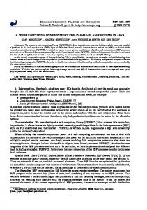
We now describe how to simulate D-BSP programs on the HMM model with a slowdown which is merely proportional to the loss of parallelism. The simulation is able to hide the memory hierarchy costs induced by the HMM access function by efficiently transforming submachine locality into temporal locality of reference. We refer to D-BSP and HMM as the guest and host machine, respectively, and restrict our attention to the simulation of D-BSP programs that end with a global synchronization (i.e., a 0-superstep), a reasonable constraint. Consider the simulation of a D-BSP program P and let µ denote the size of each D-BSP processor’s local memory, which we refer to as the processor’s context. We assume that a processor’s context also comprises the necessary buffer space for storing incoming and outgoing messages. The memory of the host machine is divided into blocks of µ cells each, with block 0 at the top of memory. At the beginning of the simulation, block j, j = 0, 1, . . . , n − 1, contains the context (i.e., the local memory) of processor Pj , but this association changes as the simulation proceeds. Let the supersteps of P be numbered consecutively, and let is be the label of the s-th superstep, with s ≥ 0 (i.e., the s-th superstep is executed independently within is -clusters). At some arbitrary point during the simulation, an is -cluster C is said to be s-ready if, for all processors in C, supersteps 0, 1, . . . , s − 1 have been simulated, while Superstep s has not been simulated yet. The simulation, whose pseudocode is given in Figure 1.1, is organized into a number of rounds, corresponding to the iterations of the while loop in the code. A round simulates the operations prescribed by a certain Superstep s for a certain s-ready cluster C, and performs a number of context swaps to prepare for the execution of the next round. The correctness of the simulation follows by showing that the two invariants given below are maintained at the beginning of each round. Let s and C be defined as in Step 1 of the round.

Invariant 1.4.2 C is s-ready.

1.4. D-BSP AND THE MEMORY HIERARCHY 1

2 3 4

27

while true do P ← processor whose context is on top of memory s ← superstep number to be simulated next for P C ← is -cluster containing P Simulate Superstep s for C if P has finished its program then exit if is+1 < is then b ← 2is −is+1 ˆ be the is+1 -cluster containing C, Let C ˆ0 . . . C ˆb−1 be its component is -clusters, and let C ˆ with C = Cj for some index j ˆ0 if j > 0 then swap the contexts of C with those of C if j < b − 1 then ˆ0 with those of C ˆj+1 swap the contexts of C

Figure 1.1: The simulation algorithm Invariant 1.4.3 The contexts of all processors in C are stored in the topmost |C| blocks, sorted in increasing order by processor number. Moreover, for any other cluster C 0 , the contexts of all processors in C 0 are stored in consecutive memory blocks (although not necessarily sorted).

It is important to observe that in order to transform the submachine locality of the D-BSP program into temporal locality of reference on the HMM, the simulation proceeds unevenly on the different D-BSP clusters. This is achieved by suitably selecting the next cluster to be simulated after each round, which, if needed, must be brought on top of memory. In fact, the same cluster could be simulated for several consecutive supersteps so to avoid repeated, expensive relocations of its processors’ contexts in memory. More precisely, consider a generic round where Superstep s is simulated for an is -cluster C. If is+1 ≥ is then no cluster swaps are performed at the end of the round, and the next round will simulate Superstep s + 1 for the topmost is+1 -cluster contained in C and currently residing on top of memory. Such a cluster is clearly (s + 1)-ready. Instead, if is+1 < is , Superstep s + 1 involves a coarser level of clustering, hence the simulation of this superstep can take place only after Superstep s has been simulated for all is -clusters that form the is+1 -cluster Cˆ containing C. Step 4 is designed to enforce this schedule. In particular, let Cˆ contain b = 2is −is+1 is -clusters, including C, which we denote by Cˆ0 , Cˆ1 , . . . , Cˆb−1 , and suppose that C = Cˆ0 is the first such is -cluster for which Superstep s is simulated. By Invariant 1.4.3, at the beginning of the round under consideration the contexts of all processors in Cˆ are at the top of memory. This

28


round starts a cycle of b phases, each phase comprising one or more simulation rounds. In the k-th phase, 0 ≤ k < b, the contexts of the processors in Cˆk are brought to the top of memory, then all supersteps up to Superstep s are simulated for these processors, and finally the contexts of Cˆk are moved back to the positions occupied at the beginning of the cycle. If the two invariants hold, then the simulation of cluster C in Step 2 can be performed as follows. First the context of each processor in C is brought in turn to the top of memory and its local computation is simulated. Then, message exchange is simulated by scanning the processors’ outgoing message buffers sequentially and delivering each message to the incoming message buffer of the destination processor. The location of these buffers is easily determined since, by Invariant 1.4.3, the contexts of the processors are sorted by processor number. The running time of the simulation algorithm is summarized in the following theorem. Theorem 1.4.4 ([7, Thm.5]) Consider a D-BSP(n, g(x), `(x)) program P, where each processor performs local computation for O (τ ) time, and there are λi i-supersteps for 0 ≤ i ≤ log n. If f (x) is (2, c)-uniform, then P can be simulated on a f (x)-HMM in P n i λ f (µn/2 ) . time O n τ + µ log i i=0 Since our main objective is to assess to what extent submachine locality can be transformed into locality of reference, we now specialize the above result to the simulation of fine-grained D-BSP programs where the local memory of each processor has constant size (i.e., µ = O (1)). In this fashion, submachine locality is the only locality that can be exhibited by the parallel program. By further constraining the D-BSP bandwidth and latency functions to reflect the HMM access function, we get the following corollary which states the linear slowdown result claimed at the beginning of the subsection. Corollary 1.4.5 If f (x) is (2, c)-uniform then any T -time fine-grained program for a DBSP(n, g(x), `(x)) with g(x) = `(x) = f (x) can be simulated in optimal time Θ (T · n) on f (x)-HMM. We note that the simulation is on-line in the sense that the entire sequence of supersteps


29

needs not be known by the processors in advance. Moreover, the simulation code is totally oblivious to the D-BSP bandwidth and latency functions g(x) and `(x).

Case studies On a number of prominent problems the simulation described above can be employed to transform efficient fine-grained D-BSP algorithms into optimal HMM strategies. Specifically, we consider the following problems. • n-MM: the problem of multiplying two

√

n×

√

n matrices on an n-processor D-BSP

using only semiring operations; • n-DFT: the problem of computing the Discrete Fourier Transform of an n-vector • 1-sorting: the special case of k-sorting, with k = 1, as defined in Section 1.2. For concreteness, we will consider the HMM access functions f (x) = xα , with 0 < α < 1, and f (x) = log x. Under these functions, upper and lower bounds for our reference problems have been developed directly for the HMM in [30]. The theorem below follows from the results in [7].

Theorem 1.4.6 There exist D-BSP algorithms for the n-MM and n-DFT problems whose simulations on the f (x)-HMM result into optimal algorithms for f (x) = xα , with 0 < α < 1, and f (x) = log x. Also, there exists a D-BSP algorithm for 1-sorting whose simulation on the f (x)-HMM results into an optimal algorithm for f (x) = xα , with 0 < α < 1 and into an algorithm with a running time which is a factor O (log n/ log log n) away from optimal for f (x) = log x.

It has to be remarked that the non-optimality of the log(x)-HMM 1-sorting is not due to an inefficiency in the simulation, but, rather, to the lack of an optimal 1-sorting algorithm for the D-BSP(n, log(x), log(x)), the best strategy known so far requiring Ω(log2 n) time. In fact, the results in [30] and our simulation imply an Ω (log n log log n) lower bound for 1sorting on D-BSP(n, log(x), log(x)) which is tighter than the previously known, trivial bound of Ω (log n).

30

CHAPTER 1. DECOMPOSABLE BSP Theorem 1.4.6 provides evidence that D-BSP can be profitably employed to obtain effi-

cient, portable algorithms for hierarchical architectures.

1.4.3

Extension to space locality

In this subsection we modify the simulation described in the previous subsection to run efficiently on the BT model which rewards both temporal and spatial locality of reference. We observe that the simulation algorithm of Figure 1.1 yields a valid BT program but it is not designed to exploit block transfer. For example, in Step 2 the algorithm brings one context at a time to the top of memory and simulates communications touching the contexts in a random fashion, which is highly inefficient in the BT framework. Since the BT model supports block copy operations only for non-overlapping memory regions, additional buffer space is required to perform swaps of large chunks of data; moreover, in order to minimize access costs, such buffer space must be allocated close to the blocks to be swapped. As a consequence, the required buffers must be interspersed with the contexts. Buffer space can be dynamically created or destroyed by unpacking or packing the contexts in a cluster. More specifically, unpacking an i-cluster involves suitably interspersing µn/2i empty cells among the contexts of the cluster’s processors so that block copy operations can take place. The structure of the simulation algorithm is identical to the one in Figure 1.1, except that the simulation of the s-th superstep for an is -cluster C is preceded (resp. followed) by a packing (resp., unpacking) operation on C’s contexts. The actual simulation of the superstep is organized into two phases: first, local computations are executed in a recursive fashion, and then the communications required by the superstep are simulated. In order to exploit both temporal and spatial locality in the simulation of local computations, processor contexts are iteratively brought to the top of memory in chunks of suitable size, and the prescribed local computation is then performed for each chunk recursively. To deliver all messages to their destinations, we make use of sorting. Specifically, the contexts of C are divided into Θ (µ|C|) constant-sized elements, which are then sorted in such a way that after the sorting, contexts are still ordered by processor number and all messages des-


31

tined to processor Pj of C are stored at the end of Pj ’s context. This is easily achieved by sorting elements according to suitably chosen tags attached to the elements, which can be produced during the simulation of local computation without asymptotically increasing the running time. The running time of the simulation algorithm is summarized in the following theorem. Theorem 1.4.7 ([7, Thm.5]) Consider a D-BSP(n, g(x), `(x)) program P, where each processor performs local computation for O (τ ) time, and there are λi i-supersteps for 0 ≤ i ≤ log n. If f (x) is (2, c)-uniform, then P can be simulated on a f (x)-BT in time P n i λ log(µn/2 ) . O n τ + µ log i i=0 We remark that, besides the unavoidable term nτ , the complexity of the sorting operations employed to simulate communications is the dominant factor in the running time. Moreover, it is important to observe that, unlike the HMM case, the complexity in the above theorem does not depend on the access function f (x), neither does it depend on the D-BSP bandwidth and latency functions g(x) and `(x). This is in accordance with the findings of [31], which show that an efficient exploitation of the powerful block transfer capability of the BT model is able to hide access costs almost completely.

Case Studies As for the HMM model we substantiate the effectiveness of our simulation by showing how it can be employed to obtain efficient BT algorithms starting from D-BSP ones. For the sake of comparison, we observe that Fact 1.4.1 implies that for relevant access functions f (x), any straightforward approach simulating one entire superstep after the other would require time ω(n) per superstep just for touching the n processor contexts, while our algorithm can overcome such a barrier by carefully exploiting submachine locality. First consider the n-MM problem. It is shown in [7] that the same D-BSP algorithm for this problem underlying the result of Theorem 1.4.6 also yields an optimal O n3/2 time algorithm for f (x)-BT, for both f (x) = log x and f (x) = xα . In general, different D-BSP bandwidth and latency functions g(x) and `(x) may promote different algorithmic strategies for the solution of a given problem. Therefore, without a strict correspondence

32


between these functions and the BT access function f (x) in the simulation, the question arises of which choices for g(x) and `(x) suggest the best “coding practices” for BT. Unlike the HMM scenario (see Corollary 1.4.5), the choice g(x) = `(x) = f (x) is not always the best. Consider, for instance, the n-DFT problem. Two D-BSP algorithms for this problem are applicable. The first algorithm is a standard execution of the n-input FFT dag and requires one i-superstep, for 0 ≤ i < log n. The second algorithm is based on a recursive √ √ decomposition of the same dag into two layers of n independent n-input subdags, and can be shown to require 2i supersteps with label (1 − 1/2i ) log n, for 0 ≤ i < log log n. On a D-BSP(n, xα , xα ) both algorithms yield a running time of O (nα ), which is clearly optimal. However, the simulations of these two algorithms on the xα -BT take time O n log2 n and O (n log n log log n), respectively. This implies that the choice g(x) = `(x) = f (x) is not effective, since the D-BSP(n, xα , xα ) does not reward the use of the second algorithm over the first one. On the other hand, D-BSP(n, log(x), log(x)) correctly distinguishes among the two algorithms, since their respective parallel running times are O log2 n and O (log n log log n). The above example is a special case of the following more general consideration. It is argued in [7] that given two D-BSP algorithms A1 , A2 solving the same problem, if the simulation of A1 on f (x)-BT runs faster than the simulation of A2 , then A1 exhibits a better asymptotic performance than A2 also on the D-BSP(n, g(x), `(x)), with g(x) = `(x) = log x, which may not be the case for other functions g(x) and `(x). This proves that DBSP(n, log x, log x) is the most effective instance of the D-BSP model for obtaining sequential algorithms for the class of f (x)-BT machines through our simulation.

1.5

Conclusions

In this chapter, we have considered the Decomposable Bulk Synchronous Parallel model of computation as an effective framework for the design of algorithms that can run efficiently on realistic parallel platforms. Having proposed a quantitative notion of effectiveness, we have shown that D-BSP is more effective than the basic BSP when the target platforms have decomposition trees with geometric bandwidth progressions. This class includes multidimen-

1.5. CONCLUSIONS

33

sional arrays and tori, as well as fat-trees with area-universal or volume-universal properties. These topologies are of particular interest, not only because they do account for the majority of current machines, but also because physical constraints imply convergence toward these topologies in the limiting technology [51]. The greater effectiveness of D-BSP is achieved by exploiting the hierarchical structure of the computation and by matching it with the hierarchical structure of the machine. In general, describing these hierarchical structures requires logarithmically many parameters in the problem and in the machine size, respectively. However, this complexity is considerably reduced if we restrict our attention to the case of geometric bandwidth and latency progressions, essentially captured by D-BSP(n, xα , xβ ) , with a small, constant number of parameters. While D-BSP is more effective than BSP with respect to multidimensional arrays, the residual loss of effectiveness is not negligible, not just in quantitative terms, but also in view of the relevance of some of the algorithms for which D-BSP is less effective. In fact, these include the d-dimensional near-neighbor algorithms frequently arising in technical and scientific computing. The preceding observations suggest further investigations to evolve the D-BSP model both in the direction of greater effectiveness, perhaps by enriching the set of partitions into clusters that can be the base of a superstep, and in the direction of greater simplicity, perhaps by suitably restricting the space of bandwidth and latency functions. In all cases, particularly encouraging are the results reported in the previous section, showing how D-BSP is well poised to incorporate refinements for an effective modeling of the memory hierarchy and providing valuable insights toward a unified framework for capturing communication requirements of computations

Acknowledgments The authors wish to thank Carlo Fantozzi, who contributed to many of the results surveyed in this work. Support for the authors was provided in part by MIUR of Italy under Project ALGO-NEXT: ALGOrithms for the NEXT generation Internet and Web and by the European Union under the FP6-IST/IP Project 15964 AEOLUS: Algorithmic Principles for

34


Building Efficient Overlay Computers

References [1] J.E. Savage. Models of Computation – Exploring the Power of Computing. Addison Wesley, Reading, MA, USA, 1998. [2] P. De la Torre and C.P. Kruskal. Submachine locality in the bulk synchronous setting. In Proc. of EUROPAR 96, LNCS 1124, pages 352–358, August 1996. [3] L.G. Valiant. A bridging model for parallel computation. Communications of the ACM, 33(8):103–111, August 1990. [4] G. Bilardi, A. Pietracaprina, and G. Pucci. A quantitative measure of portability with application to bandwidth-latency models for parallel computing. In Proc. of EUROPAR 99, LNCS 1685, pages 543–551, September 1999. [5] G. Bilardi, C. Fantozzi, A. Pietracaprina, and G. Pucci. On the effectiveness of DBSP as a bridging model of parallel computation. In Proc. of the Int. Conference on Computational Science, LNCS 2074, pages 579–588, 2001. [6] C. Fantozzi, A. Pietracaprina, and G. Pucci. A general PRAM simulation scheme for clustered machines. Intl. Journal of Foundations of Computer Science, 14(6):1147–1164, 2003. [7] C. Fantozzi, A. Pietracaprina, and G. Pucci. Translating submachine locality into locality of reference. Journal of Parallel and Distributed Computing, 66:633–646, 2006. Special issue on 18th IPDPS. [8] T.H. Cormen, C.E. Leiserson, R.L. Rivest, and C. Stein. Introduction to Algorithms. McGraw-Hill/MIT Press, 2nd edition, 2001. [9] S.A. Cook and R.A. Reckhow. Time bounded random access machines. Journal of Computer and System Sciences, 7:354–375, 1973. [10] R.P. Brent. The parallel evaluation of general arithmetic expressions. Journal of the ACM, 21(2):201–208, 1974. [11] S. Fortune and J. Wyllie. Parallelism in random access machines. In Proc. of the 10th ACM Symp. on Theory of Computing, pages 114–118, 1978. [12] L.M. Goldschlager. A unified approach to models of synchronous parallel machines. Journal of the ACM, 29:1073–1086, 1982. [13] R.M. Karp and V. Ramachandran. Parallel algorithms for shared-memory machines. In Handbook of Theoretical Computer Science, Volume A: Algorithms and Complexity, pages 869–942. Elsevier and MIT Press, 1990. [14] J. JáJá. An Introduction to Parallel Algorithms. Addison Wesley, Reading MA, 1992. [15] F.T. Leighton. Introduction to Parallel Algorithms and Architectures: Arrays • Trees • Hypercubes. Morgan Kaufmann, San Mateo, CA, 1992. [16] M.C. Pease. The indirect binary n-cube microprocessor array. IEEE Trans. on Computers, C-26(5):458–473, May 1977. [17] H.S. Stone. Parallel processing with the perfect shuffle. IEEE Trans. on Computers, C-20(2):153–161, Feb. 1971. [18] F.P. Preparata and J. Vuillemin. The cube-connected-cycles: A versatile network for parallel computation. Communications of the ACM, 24(5):300–309, May 1981. [19] C.E. Leiserson. Fat-trees: universal networks for hardware-efficient supercomputing. IEEE Trans. on Computers, C-34(10):892–901, October 1985. [20] E. Upfal and A. Widgerson. How to share memory in a distributed system. Journal of the ACM, 34(1):116–127, 1987.

1.5. CONCLUSIONS

35

[21] A. Pietracaprina, G. Pucci, and J. Sibeyn. Constructive, deterministic implementation of shared memory on meshes. SIAM Journal on Computing, 30(2):625–648, 2000. [22] M. Hall Jr. Combinatorial Theory. John Wiley & Sons, New York NY, second edition, 1986. [23] D.E. Culler, R. Karp, D. Patterson, A. Sahay, E. Santos, K.E. Schauser, R. Subramonian, and T.V. Eicken. LogP: A practical model of parallel computation. Communications of the ACM, 39(11):78–85, November 1996. [24] G. Bilardi, K.T. Herley, A. Pietracaprina, G. Pucci, and P. Spirakis. BSP vs LogP. Algorithmica, 24:405–422, 1999. Special Issue on Coarse Grained Parallel Algorithms. [25] G. Bilardi, K. Herley, A. Pietracaprina, and G. Pucci. On stalling in LogP. Journal of Parallel and Distributed Computing, 65:307–312, 2005. [26] A. Aggarwal, A.K. Chandra, and M. Snir. Communication complexity of PRAMs. Theoretical Computer Science, 71:3–28, 1990. [27] P.B. Gibbons, Y. Matias, and V. Ramachandran. Can a shared-memory model serve as a bridging-model for parallel computation? Theory of Computing Systems, 32(3):327– 359, 1999. [28] M. Snir and J.A. Solworth. Ultracomputer note 29. The Ultraswitch – A VLSI network node for parallel processing. Technical report, Courant Institute, New York University, 1984. [29] G.L.-T. Chiu, M. Gupta, and A.K. Royyuru, editors. Blue Gene. Special issue of IBM Journal of Research and Development 49(2/3), 2005. [30] A. Aggarwal, B. Alpern, A.K. Chandra, and M. Snir. A model for hierarchical memory. In Proc. of the 19th ACM Symp. on Theory of Computing, pages 305–314, 1987. [31] A. Aggarwal, A.K. Chandra, and M. Snir. Hierarchical memory with block transfer. In Proc. of the 28th IEEE Symp. on Foundations of Computer Science, pages 204–216, 1987. [32] G. Bilardi, K. Ekanadham, and P. Pattnaik. Computational power of pipelined memory hierarchies. In Proc. of the 13th ACM Symp. on Parallel Algorithms and Architectures, pages 144–152, 2001. [33] G. Bilardi, K. Ekanadham, and P. Pattnaik. Optimal organizations for pipelined hierarchical memories. In Proc. of the 14th ACM Symp. on Parallel Algorithms and Architectures, pages 109–116, 2002. [34] M.T. Goodrich. Communication-efficient parallel sorting. SIAM Journal on Computing, 29(2):416–432, 1999. [35] C. Fantozzi, A. Pietracaprina, and G. Pucci. Implementing shared memory on clustered machines. In Proc. of 2nd International Parallel and Distributed Processing Symposium, 2001. [36] G. Baudet and D. Stevenson. Optimal sorting algorithms for parallel computers. IEEE Trans. on Computers, C-27(1):84–87, January 1978. [37] B.H.H. Juurlink and H.A.G. Wijshoff. A quantitative comparison of parallel computation models. In Proc. of the 8th ACM Symp. on Parallel Algorithms and Architectures, pages 13–24, June 1996. [38] A. Czumaj, F. Meyer auf der Heide, and V. Stemann. Shared memory simulations with triple-logarithmic delay. In Proc. of the 3rd European Symposium on Algorithms, pages 46–59, 1995. [39] A.G. Ranade. How to emulate shared memory. Journal of Computer and System Sciences, 42:307–326, 1991. [40] J.L. Carter and M.N. Wegman. Universal classes of hash functions. Journal of Computer and System Sciences, 18:143–154, 1979. [41] K. Mehlhorn and U. Vishkin. Randomized and deterministic simulations of PRAMs by parallel machines with restricted granularity of parallel memories. Acta Informatica, 21:339–374, 1984.

36


[42] F.T. Leighton and S. Rao. Multicommodity max-flow min-cut theorems and their use in designing approximation algorithms. Journal of the ACM, 46(6):787–832, 1999. [43] F.T. Leighton, B.M. Maggs, and A.W. Richa. Fast algorithms for finding O(congestion + dilation) packet routing schedules. Combinatorica, 19(3):375–401, 1999. [44] U. Vishkin. Can parallel algorithms enhance serial implementation? Communications of the ACM, 39(9):88–91, 1996. [45] J.F. Sibeyn and M. Kaufmann. BSP-like external-memory computation. In Proc. of 3rd CIAC, LNCS 1203, pages 229–240, 1999. [46] F. Dehne, W. Dittrich, and D. Hutchinson. Efficient external memory algorithms by simulating coarse-grained parallel algorithms. Algorithmica, 36(2):97–122, 2003. [47] F. Dehne, D. Hutchinson, D. Maheshwari, and W. Dittrich. Bulk synchronous parallel algorithms for the external memory model. Theory of Computing Systems, 35(6):567– 597, 2002. [48] C. Fantozzi, A. Pietracaprina, and G. Pucci. Seamless integration of parallelism and memory hierarchy. In Proc. of 29th Int. Colloquium on Automata, Languages and Programming, LNCS 2380, pages 856–867, July 2002. [49] G. Bilardi and E. Peserico. A characterization of temporal locality and its portability across memory hierarchies. In Proc. of 28th Int. Colloquium on Automata, Languages and Programming, LNCS 2076, pages 128–139, 2001. [50] J.S. Vitter and E.A.M. Shriver. Algorithms for parallel memory II: Hierarchical multilevel memories. Algorithmica, 12(2/3):148–169, 1994. [51] G. Bilardi and F.P. Preparata. Horizons of parallel computing. Journal of Parallel and Distributed Computing, 27:172–182, 1995.

Handbook of Parallel Computing: Models, Algorithms, and ... - DEI UniPd

Handbook of Parallel Computing: Models, Algorithms, and ... - DEI UniPd

Suggest Documents

pdf-1470\handbook-of-parallel-computing-models-algorithms-and ...

Convention Paper - DEI UniPd

Cache-Oblivious Simulation of Parallel Programs - DEI UniPd

Self-splitting of workload in parallel computation - DEI UniPd

NETTAB08_Francesco Sambo - DEI UniPd

Untitled - DEI UniPd

Convention Paper - DEI UniPd

Engineering Parallel Algorithms for Community ... - Parallel Computing

Parallel Processing Letters &c World Scientific Publishing ... - DEI UniPd

Parallel Computing: Architectures, Algorithms and Applications - Unipi

Debugging with Eclipse - DEI UniPd

Fountain Reprogramming Protocol - DEI UniPd

Integrating physically based sound models in a ... - DEI UniPd

A General Linear Mixed Models Approach to Study ... - DEI UniPd

Proceedings Template - WORD - DEI UniPd

Low-level models: resonators, interactions, surface textures - DEI UniPd

DETERMINISTIC BRANCH-AND-BOUND ON ... - DEI UniPd

PHYSICALLY-BASED SYNTHESIS OF NONLINEAR ... - DEI UniPd

Parallel-Algorithms-Numerical-Scientific-Computing-1584889454 ...

Grid computing for parallel bioinspired algorithms - CiteSeerX

A WEB COMPUTING ENVIRONMENT FOR PARALLEL ALGORITHMS

Parallel algorithms for large scale econometric models

Obtaining Performance Measures through ... - DEI UniPd

Approximating the split closure - DEI UniPd