Congress on Evolutionary Computation (CEC), Oregon, USA, 2004: 2012-2016
Handling Equality Constraints by Adaptive Relaxing Rule for Swarm Algorithms Xiao-Feng Xie Institute of Microelectronics, Tsinghua University, Beijing 100084, P. R. China Email:
[email protected]
Wen-Jun Zhang Institute of Microelectronics, Tsinghua University, Beijing 100084, P. R. China Email:
[email protected]
Abstract- The adaptive constraints relaxing rule for swarm algorithms to handle with the problems with eqaulity constraints is presented. The feasible space of such problems may be similiar to ridge function class, which is hard for applying swarm algorithms. To enter the solution space more easily, the relaxed quasi feasible space is introduced and shrinked adaptively. The experimental results on benchmark functions are compared with the performance of other algorithms, which show its efficiency.
I. INTRODUCTION A problem with equality constraints can be defined as: Miniminze : f ( xG ) G Subject to: g j ( x ) ≤ 0 (1 ≤ j ≤ m 0 , j ∈ ] ) G h j ( x ) = 0 ( m0 + 1 ≤ j ≤ m , j ∈ ] )
(1)
G
where x = ( x1 ,..., xd ,..., xD ) and the search space (S) is a D-dimensional space bounded by all the parametric constraints xd ∈ [ l d , u d ]. f is objective function, gi and hj are inequality and equality constraints, respectively. The set of points, which satisfying all the constraints, is denoted as feasible space ( S F ), and then the infeasible space is S I =S F ∩ S . Normally, an equality constraint is transformed into an inequality one, i.e. g j + m0 =| h j | −ε h , j ≤ 0 , for some small
violation values ε h ≥ 0 [4, 6, 7, 13]. Swarm algorithms are behavioral models based on the concepts of social swarm that belong to learning paradigms [5]. Each swarm comprises a society of autonomous agents, which each agent [2] is worked by executing the simple action rules according available information in iterated learning cycles. Existing examples include particle swarm optimization (PSO) [3, 10, 15], differential evolution (DE) [16] and their hybrid [17], etc. For swarm algorithms, the information is represented by G each point x ∈ S , which its goodness is evaluated by the G G goodness function F( x ). Suppose for a point x * , there G G G G G exists F (x * ) ≤ F ( x ) for ∀x ∈ S , then x * and F( x ) are separately the global optimum point and its value. In general, the goal is to find point(s) that belong to the G G G G solution space SO = {x ∈ S F | F∆ ( x ) = F ( x ) − F ( x * ) ≤ ε O } G instead of the x * , where ε O is a small positive value.
De-Chun Bi Department of Environmental Engineering, Liaoning University of Petroleum & Chemical Technology Fushun, Liaoning, 113008, P. R. China
G The goodness function F ( x ) is encoded by constrainthandling methods that applied on the problem [12]. In order to avoiding the laborious settings for the penalty coefficients [4, 13], and without requiring a starting point in S F [8], the method that following Deb’s criteria [6] is applied on swarm algorithms for the problems with inequality constraints successfully [11, 17]. However, it is still difficulty to deal with equality constraints [8], especially when the violation values are very small [17]. This paper intends to handling with equality constraints for swarm algorithms. In the section 2, the details on swarm algorithms are introduced. Then in the section 3, the ridge function class problem [1, 13] is analysized, which shows that it is hard for swarm algorithms. In the section 4, the basic constraints handling (BCH) rule, which is following Deb’s criteria, is introduced. And then the adaptive constraints relaxing (ACR) rule is then studied, since the BCH rule may bring the problem with eqaulity constraints into ridge function class. Then the method is applied to three benchmark functions [12], and the experimental results are compared with those of existing algorithms [7, 13], which illustrate the significant performance improvement.
II. SWARM ALGORITHMS In swarm algorithms, each agent is worked in iterated learning cycles. Supposing the number of agents in a swarm is N, and the total number of learning cycles is T, then at the tth ( 1 ≤ t ≤ T , t ∈ ] ) learning cycle, each agent is activated in turn, which generates-and-tests a new point based on its own experience and the social sharing information. For the convenience of discussion, for the ith ( 1 ≤ i ≤ N , i ∈ ] ) agent, the point with the best goodness value generated in its past learning cycles is defined as G pi (t ) . The point with the best goodness value in the set G G { pi ( t ) | 1 ≤ i ≤ N , i ∈ ] } is defined as g ( t ) , which is often the main source of the social sharing information. The total evalution times are TE= N·T.
A. Particle swarm (PS) agent Particle swarm agent, called particle [10], generates G x ( t +1) according to the historical experiences of its own and its colleagues, for the dth dimension [15]:
vd ( t +1) = w ⋅ vd ( t ) + c1 ⋅ U \ () ⋅ ( pd ( t ) − xd ( t ) )
(2)
+ c2 ⋅ U \ () ⋅ ( g d ( t ) − xd ( t ) ) xd ( t +1) = xd ( t ) + vd ( t +1)
G G center is between pi and g , and the variation strength is with consensus on the diversity of swarm. As shown in G G G G figure 1, SV ( xA , xB ) is a typical variation space as g = x A G G and pi = xB .
where w is inertia weight, U \ () is a random real value between 0 and 1. The default parameter values include: c1 = c2 = 2 . G G SV ( xA , xB )
B. Differential evolution (DE) agent Differential evolution agent generates a new point G G G ( t +1) G (t ) k (t +1) for updating its p (t +1) . At first, it sets xDE =p , and DR = U ] (1, D ) is a random integer value within [1, D]. For the dth dimension [16, 17], if U \ () < CR or d = DR , then the following rule is applied: ( t +1) (t ) xDE + SF ⋅ ∆ (NtV) , d ,d = gd
(3)
where CR ∈ [0,1] is crossover factor, DR ensures the variation at least in one dimension, SF is scaling factor. G G G G G ∆ (NtV) = ∑1NV ∆1(t ) , and ∆1( t ) = pU ] (1, N ) ( t ) − pU ] (1, N ) ( t ) is called difference vector. The default parameter values include: G (t +1) G )≤F( p (t ) ), then NV =2, SF= 1/ NV =0.5. At last, if F( xDE G (t +1) G (t +1) := xDE . it sets p C. Combined DEPS agent
Agent-based modeling provides a natural framework for tuning the rules of each agent [2]. The action rules of DEPS agent [17] is the combination of a DE rule and a PS rule. At the odd t, the PS rule is activated for updating its G G G v ( t +1) , x ( t +1) and p (t +1) , then at the even t, the DE rule is G G G activated for updating its pi ( t +1) . Notes the v (t ) and x ( t ) that required by PS rule are not changed by DE rule. G G However, both rules share with same p (t ) and g ( t ) , which allows them coupling with each other. III. RIDGE FUNCTION CLASS The ridge function class problem may be regarded as extensions of the sphere model breaking its total rotational symmetry in some dimensions of the parameter space [1]. G G G As shown in figure 1, S B ( x A ) = {F ( x ) ≤ F ( x A )} is an example of ridge function, SO is the solution space. For a G point x A , II and IO is the improvement interval [13], i.e. the possible interval for improving its goodness, and the distance to SO along with a single dimension, respectively. The significant feature of ridge function is that the ratio II /IO is small due to the large eccentricities. The action rules of agents in swarm provide a selfadaptive bell-shaped variations [9, 17], which the gravity
G S B ( xA )
G xB
G xA Figure 1. Ridge function class problem.
If an action rule generates new points by modifying only one dimension of current point, then it is obviously that small II/IO results in an increase of the difficulty for convergence, due to the zigzag path in small steps [13]. The common case is that an action rule generates new points by varying several dimensions of current point. It seems that the implicit combination operations by the G G action rules may accelerate the convergence, as the ( p - g ) is in suitable direction and enough variation strength. However, as the variation strength is large, it has small possibility for keeping in the direction of ridge axis. Then G G G G the ratio ( S B ( g ) ∩ SV ( p, g )) / S B ( g ) is very small, which G most trails cannot enter S B ( g ) . Despite of those invalid G trails, the improving p often satisfies the short-term goal (increasing goodness by reducing the variation strength) rather than the long-term goal (finding suitable variation strength along the ridge axis for entering the SO). The G G magnitude of ( p - g ) is varying to the magnitude of II as G entering S B ( g ) . As II/IO is small, it requires many steps for entering the SO. Moreover, for the bell-shaped variations, the large adjustments are possible, but are much less than the small adjustments. During the many small steps, it has G great probability that the agents are clustered near g (t ) at a certain step and lost the diversity as the large variation are not accepted. Then the variation strength, which is with G G consensus on the diversity of p and g , becomes small, and then the swarm is easily converged prematurely due to the self-adaptation mechanism. For problems with equality constraints, if the violation values are very small, then the SF becomes very narrow. If it is cut into several segments, then some of them have great probability to be in ridge function class landscape. The many directions for the ridge axes of multiple segments increase the difficulty much more.
IV. BASIC CONSTRAINTS HANDLING (BCH) G The total goodness function F ( x ) includes two parts, m G G G G where FOBJ ( x ) = f ( x ) and FCON ( x ) = ∑ rjG j ( x ) are the j =1
goodness functions for objective funtion and constraints, G G respectively. Here G j ( x ) = max(0, g j ( x )) [4], and rj are positive weight factors, which default value is equal to 1. The basic constraints handling (BCH) rule for goodness G evaluation is realized by comparing any two points x A , G G G xB , F ( x A ) ≤ F ( xB ) when G G FCON ( xA ) < FCON ( xB ) OR G G G G FOBJ ( x A ) ≤ FOBJ ( xB ) AND FCON ( xA ) = FCON ( xB )
normally. In P, the number G FCON ( pi (t ) ) > ε R(t ) is defined as Nε(t ) .
in SF, the one having smaller FOBJ is preferred; c) among two points in SI, the one having smaller FCON is preferred. V. ADAPTIVE CONSTRAINTS RELAXING (ACR) For the convenience of discussion, the probability for G changing x from space SX to SY is defined as P ( S X → SY ) . The searching path of the BCH rule is S I → S F → SO . Then the problems with equality constraints are hard problems for swarm algorithms since the P ( S F → SO ) can be very small as SF is in ridge function class. In this paper, the goodness landscape is transformed by constraints relaxing rule so as to match swarm algorithms. G The quasi feasible space is defined S F' = {FCON ( x ) ≤ ε R } ,
IF(rN(t ) ≤ rl ) THEN ε R(t +1) = βu ⋅ ε R(t ) (t ) N
IF(r
' F
It means that among two points in S , the one with smaller FOBJ is preferred. Then the searching path becomes S I → S F' → SO' . Since S F ⊆ S F' , it is obviously
≥ ru ) THEN ε
( t +1) R
= βl ⋅ ε
S F' , 0 ≤ rl < ru ≤ 1 , 0 < βl < 1 < β u .
The ε R(t ) is not varied as rN( t ) ∈ (rl , ru ) . If the ε R( t ) is large G at the end of learning cycles, then g (T ) may even not enter the SO . Hence it is necessarily to prevent the ε R(t ) from stagnating for many learning cycles, especially for the cases that the elements in KO are hardly to be changed. The forcing sub-rule forces the ε R(t ) |t →T → 0 : IF(t ≥ tth ) THEN ε R (t +1) = β f ⋅ ε R( t )
The default parameter values include: rl=0.25, ru=0.75,
β f = β l =0.618, βu =1.382, and tth = 0.5 ⋅ T .
G For each learning cycle, the g ( t ) is reevaluated among G the { pi (t ) | 1 ≤ i ≤ N , i ∈ ] }, as the ε R( t ) is updated.
VI. TEST FUNCTIONS SUITE Three benchmark functions with equality constraints, called G3, G5, G11, G13, were described in [12, 13]. A. G3 D G Minimum: f ( x ) = − d d / 2 ∏ xd d =1
D
∑x
2 d
−1 = 0
P ( S F → SO ) , P ( S F' → SO' ) can increase dramaticly by the
where D=10 and 0 ≤ xd ≤ 1 (d = 1, …,D).
enlarged II/IO. Then it has P( S I → SO' ) ≥ P( S I → SO ) . G G Of course, x ∈ SO' does not necessarily mean x ∈ SO .
B. G5
decreasing ε R for increasing ( S ∩ SO ) SO . For the extremal case, when ε R =0, it has SO' = SO . The adjusting of ε R( t ) is referring to a data repository P
G
= { pi ( t ) | 1 ≤ i ≤ N , i ∈ ] }, which is updated frequently,
(7)
where 0 < β f < 1 , and 0 ≤ tth ≤ T .
subject to:
' O
(6)
(t ) R
that P( S I → S F' ) ≥ P( S I → S F ) . Besides, comparing with
However, the searching path SO' → SO can be built by
with
where rN( t ) = Nε( t ) / N is the ratio of the points inside the
where ε R ≥ 0 is the relaxing threshold value, and its corresponding quasi solution space is defined as SO' , then an additional rule is applied on equation (4): G G (5) FCON ( x ) = max(ε R , FCON ( x ))
points
Initially, the ε R (0) is set as maximum FCON value in K O . Then the adaptive relaxing (ACR) rule is employed for ensuring ε R(t ) → 0 , by the following combined rules: a) the basic ratio-keeping sub-rules; b) the forcing sub-rule. The basic ratio-keeping sub-rules try to keep a balance between the points inside and outside the S F' :
(4)
The BCH rule is following Deb’s criteria [6]: a) any G G x ∈ S F is preferred to any x ∉ S F ; b) among two points
of
d =1
Minimize: G f ( x ) = 3 x1 +0.000001 x13 +2 x2 +0.000002/3 x23 subject to: x4 - x3 +0.55 ≥ 0, x3 - x4 +0.55 ≥ 0, 1000sin(- x3 -0.25)+1000sin(- x4 -0.25)+984.8- x1 = 0,
1000sin( x3 -0.25)+1000sin( x3 - x4 -0.25)+984.8- x2 = 0, 1000sin( x4 -0.25)+1000sin( x4 - x3 -0.25)+1294.8 = 0.
TE=1.4E5. For other algorithm parameters, the default values were used. 100 runs were done for each function.
where 0 ≤ xd ≤ 1200 (d=1, 2), -0.55 ≤ xd ≤ 0.55 (d =3, 4). C. G11
G Minimize: f ( x ) = x12 +( x2 -1)2 subject to:
x2 - x12 = 0.
where -1 ≤ xd ≤ 1 (d=1, 2). D. G13 G Minimize: f ( x ) = e x1 x2 x3 x4 x5 subject to:
5
∑x d =1
2 d
− 10 = 0 ,
x2 x3 − 5 x4 x5 = 0 ,
x + x +1 = 0 . where -2.3 ≤ xd ≤ 2.3 (d=1, 2), -3.2 ≤ xd ≤ 3.2 ( i=3, 4, 5). 3 1
3 2
VII. RESULTS AND DISCUSSIONS The violation value determines the difficult of problems. For the larger violation value, which is ε h =1E-3, there have already been well solved [11, 17]. Here we only perform experiments on the smaller violation value, which is ε h =1E-4, as in the literatures [7, 13]. Table 1 lists the summary of F* (also is achieved as ε h =1E-4) and the mean best fitness value (FB) by two published algorithms: a) (30, 200)-evolution strategy (ES) with stochastic ranking (SR) technique [13], T=1750, then TE=3.5E5; and b) genetic algorithm (GA) [7], which N=70, T=2E4, then TE=1.4E6. TABLE 1. EXISTING RESULTS FOR TEST PROBLEMS G3 G5 G11 G13 F* 1.0005 5126.497 0.7499 0.053942 ES [13] 1 5128.881 0.75 0.067543 GA [7] 0.9999 5432.08 0.75 -
Table 2 to 4 summary the mean results by for swarm algorithms in three kinds of constraint-handling methods: a) BCH rule; b) ACR#1, which without the forcing subrule; and c) ACR#2, which with the forcing sub-rule, respectively. The values in the parentheses describe the number of runs that are failed in entering SF, and the FB is calculated by the successful runs only. The boundary constraints are handled by periodic mode [17]. The number of agent was set as N=70. CR was fixed as 0.9 for the DE rule, and w was fixed as 0.4 for the PS rule to achieve fast convergence. For BCH rule, the learning cycles of all cases were set as T=5E3, then TE=3.5E5, which were same as ES in table 1. For ACR rules, for G3, T=5E3, then TE=3.5E5; for G5, G11 and G13, T=2E3, then
DE PS DEPS
TABLE 2. RESULTS BY BCH RULE G3 G5 G11 G13 0.3985 5133.834 0.75056 0.52800 0.8364 5334.97(12) 0.74992 1.10423 0.9849 5130.864 0.74990 0.51065
TABLE 3. RESULTS BY ACR#1 RULE (WITHOUT THE FORCING SUB-RULE) G3 G5 G11 G13 DE 0.79256 5126.497(3) 0.74990 0.08637(67) PS 1.00040 5129.328(80) 0.74990 0.20791(73) DEPS 1.00045 5126.497(1) 0.74990 0.097046 TABLE 4. RESULTS BY ACR#2 RULE (WITH THE FORCING SUB-RULE) G3 G5 G11 G13 DE 0.79854 5126.500 0.74990 0.22268(6) PS 1.00036 5131.188(1) 0.74990 0.097855 DEPS 1.00050 5126.497 0.74990 0.066257
Table 2 lists the results by the swarm algorithms in BCH rule, which G3 and G5 were also listed in [17]. Compared with table 1, it can be found that most results were not satisfied, which only DE and DEPS performed better than GA, but worse than ES for G5, and swarm algorithms performed similar to ES and GA for G11. Table 3 lists the results by the swarm algorithms in ACR#1, which without the forcing sub-rule. Compared with the results in table 2, the results for G3 and G11 are significant better, and for G5, G13, there have more failed runs although the mean results for successful runs are better. It means that the ACR#1 has the capability for improving the performance of swarm algorithms. The results for G3 and G11, especially for PS and DEPS, seem to be comparable with that of table 1. However, the results may not enter the SO , even not enter the SF, due to the stagnated ε R( t ) in some runs. Table 4 lists the results by the swarm algorithms in ACR#2, which with the forcing sub-rule. It can be found that the forcing sub-rule eliminated the failed runs. All the results were better than the results in BCH rule. The DE performed not so good for G3 and G13, and the PS performed not so good for G5. However, the results by DEPS were better than the results by existing algorithms as listed in table 1. TABLE 5.STANDARD DEVIATION FOR TEST PROBLEMS G3 G5 G11 G13 ES [13] 1.9E-04 3.5E+00 8.0E-05 3.1E-02 GA [7] 7.5E-05 3.9E+03 0.0E+00 DEPS 8.12E-07 1.41E-10 0.0E+00 6.78E-2
Table 5 summaries the standard deviations of the results by ES[13], GA [7], and DEPS in ACR#2. It can also be shown that DEPS in ACR#2 has smaller standard deviations than ES[13] and GA [7], except for G13. It is also worthy to compare stochastic ranking (SR) technique [13] with ACR Rule, since both of them achieved good results by transforming the landscape of problem. As mentioned by Farmani and Wright [7]: “The stochastic ranking technique has the advantage that it is simple to implement, but it can be sensitive to the value of its single control parameter.” Besides, the SR technique is not suitable for current swarm algorithms, since it brings G too much randomicity on deciding the g ( t ) from the stochastic landscape. The ACR rule avoids such problem, since the landscape by it is fixed in one learning cycle, although it may be varied along with the learing cycles. VIII. CONCLUSIONS Swarm algorithms are behavioral models based on the concepts of social swarm. Each agent in the swarm is worked by executing the action rules, which provide a self-adaptive bell-shaped variations with consensus on the diversity of swarm, in iterated learning cycles. However, the analysis shows such self-adaption mechanism may be hard for the SF of the problems with eqaulity constraints that in ridge function class. The adaptive constraints relaxing (ACR) rule is presented for swarm algorithms to handle with the problems with eqaulity constraints. The relaxed quasi feasible space is introduced and shrinked adaptively, so as to enter the solution space at the end of evolution. The experimental results on benchmark functions is compared with the performance of other algorithms, which shows it can achieve better results in less evalution times. REFERENCES [1] Beyer H-G. On the performance of (1, λ)-evolution strategies for the ridge function class. IEEE Trans. Evolutionary Computation. 2001, 5 (3): 218-235 [2] Bonabeau E. Agent-based modeling: methods and techniques for simulating human systems. Proc. Natl. Acad. Sci. USA. 2002, 99 (s3): 7280–7287 [3] Clerc M, Kennedy J. The particle swarm - explosion, stability, and convergence in a multidimensional complex space. IEEE Trans. Evolutionary Computation, 2002, 6(1): 58-73 [4] Coello C A C. Theoretical and numerical constraint-handling techniques used with evolutionary algorithms: a survey of the state of the art. Computer Methods in Applied Mechanics and Engineering, 2002, 191(11-12): 1245-1287 [5] de Castro L N. Immune, swarm, and evolutionary algorithms. II. Philosophical comparisons, Int. Conf. on Neural Information Processing, Orchid, Singapore, 2002: 1469-1473
[6] Deb K. An efficient constraint handling method for genetic algorithms. Computer Methods in Applied Mechanics and Engineering, 2000, 186(2-4): 311-338 [7] Farmani R, Wright J A. Self-adaptive fitness formulation for constrained optimization. IEEE Trans. Evolutionary Computation. 2003, 7 (5): 445-455 [8] Hu X H, Eberhart R C, Shi Y H. Engineering optimization with particle swarm. IEEE Swarm Intelligence Symposium, Indianapolis, IN, USA, 2003: 53-57 [9] Kennedy J. Bare bones particle swarms. IEEE Swarm Intelligence Symposium, Indianapolis, IN, USA, 2003: 80-87 [10] Kennedy J, Eberhart R C. Particle swarm optimization. IEEE Int. Conf. on Neural Networks, Perth, Australia, 1995: 19421948 [11] Lampinen J. A constraint handling approach for the differential evolution algorithm. Congress on Evolutionary Computation, 2002: 1468-1473 [12] Michalewicz Z, Schoenauer M. Evolutionary algorithms for constrained parameter optimization problems. Evolutionary Computation. 1996, 4 (1): 1-32 [13] Runarsson T P, Yao X. Stochastic ranking for constrained evolutionary optimization. IEEE Trans. Evolutionary Computation, 2000, 4(3): 284-294 [14] Salomon R. Re-evaluating genetic algorithm performance under coordinate rotation of benchmark functions. Biosystems. 1996, 39 (3): 263-278 [15] Shi Y H, Eberhart R C. Empirical study of particle swarm optimization. Congress on Evolutionary Computation, Washington DC, USA, 1999: 1945-1950 [16] Storn R, Price K. Differential evolution - a simple and efficient heuristic for global optimization over continuous spaces. J. Global Optimization, 1997, 11(4): 341–359 [17] Zhang W J, Xie X F. DEPSO: hybrid particle swarm with differential evolution operator. IEEE Int. Conf. on Systems, Man and Cybernetics, Washington DC, USA, 2003: 38163821