The data are missing completely at random (MCAR) if the ... That means that, if there is missing data on Y, one must specify how the probability that Y is missing.
SAS Global Forum 2012
Statistics and Data Analysis
Paper 312-2012
Handling Missing Data by Maximum Likelihood Paul D. Allison, Statistical Horizons, Haverford, PA, USA ABSTRACT Multiple imputation is rapidly becoming a popular method for handling missing data, especially with easy-to-use software like PROC MI. In this paper, however, I argue that maximum likelihood is usually better than multiple imputation for several important reasons. I then demonstrate how maximum likelihood for missing data can readily be ® implemented with the following SAS procedures: MI, MIXED, GLIMMIX, CALIS and QLIM.
INTRODUCTION Perhaps the most universal dilemma in statistics is what to do about missing data. Virtually every data set of at least moderate size has some missing data, usually enough to cause serious concern about what methods should be used. The good news is that the last twenty five years have seen a revolution in methods for handling missing data. The new methods have much better statistical properties than traditional methods, while at the same time relying on weaker assumptions. The bad news is that these superior methods have not been widely adopted by practicing researchers. The most likely reason is ignorance. Many researchers have barely even heard of modern methods for handling missing data. And if they have heard of them, they have little idea how to go about implementing them. The other likely reason is difficulty. Modern methods can take considerably more time and effort, especially with regard to start-up costs. Nevertheless, with the development of better software, these methods are getting easier to use every year. There are two major approaches to missing data that have good statistical properties: maximum likelihood (ML) and multiple imputation (MI). Multiple imputation is currently a good deal more popular than maximum likelihood. But in this paper, I argue that maximum likelihood is generally preferable to multiple imputation, at least in those situations where appropriate software is available. And many SAS users are not fully aware of the available procedures for using maximum likelihood to handle missing data. In the next section, we’ll examine some assumptions that are commonly used to justify methods for handling missing data. In the subsequent section, we’ll review the basic principles of maximum likelihood and multiple imputation. After I present my arguments for the superiority of maximum likelihood, we’ll see how to use several different SAS procedures to get maximum likelihood estimates when data are missing.
ASSUMPTIONS To make any headway at all in handling missing data, we have to make some assumptions about how missingness on any particular variable is related to other variables. A common but very strong assumption is that the data are missing completely at random (MCAR). Suppose that only one variable Y has missing data, and that another set of variables, represented by the vector X, is always observed. The data are missing completely at random (MCAR) if the probability that Y is missing does not depend on X or on Y itself (Rubin 1976). To represent this formally, let R be a “response” indicator having a value of 1 if Y is missing and 0 if Y is observed. MCAR means that
Pr( R = 1 | X , Y ) = Pr( R = 1) If Y is a measure of delinquency and X is years of schooling, MCAR would mean that the probability that data are missing on delinquency is unrelated to either delinquency or schooling. Many traditional missing data techniques are valid only if the MCAR assumption holds. A considerably weaker (but still strong) assumption is that data are missing at random (MAR). Again, this is most easily defined in the case where only a single variable Y has missing data, and another set of variables X has no missing data. We say that data on Y are missing at random if the probability that Y is missing does not depend on Y, once we control for X. Formally, we have
Pr( R = 1 | X , Y ) = Pr( R = 1 | X ) where, again, R is the response indicator. Thus, MAR allows for missingness on Y to depend on other variables that are observed. It just cannot depend on Y itself (after adjusting for the observed variables). Continuing our example, if Y is a measure of delinquency and X is years of schooling, the MAR assumption would be satisfied if the probability that delinquency is missing depends on years of schooling, but within each level of schooling, the probability of missing delinquency does not depend on delinquency.
1
SAS Global Forum 2012
Statistics and Data Analysis
In essence, MAR allows missingness to depend on things that are observed, but not on things that are not observed. Clearly, if the data are missing completely at random, they are also missing at random. It is straightforward to test whether the data are missing completely at random. For example, one could compare men and women to test whether they differ in the proportion of cases with missing data on income. Any such difference would be a violation of MCAR. However, it is impossible to test whether the data are missing at random, but not completely at random. For obvious reasons, one cannot tell whether delinquent children are more likely than nondelinquent children to have missing data on delinquency. What if the data are not missing at random (NMAR)? What if, indeed, delinquent children are less likely to report their level of delinquency, even after controlling for other observed variables? If the data are truly NMAR, then the missing data mechanism must be modeled as part of the estimation process in order to produce unbiased parameter estimates. That means that, if there is missing data on Y, one must specify how the probability that Y is missing depends on Y and on other variables. This is not straightforward because there are an infinite number of different models that one could specify. Nothing in the data will indicate which of these models is correct. And, unfortunately, results could be highly sensitive to the choice of model. A good deal of research has been devoted to the problem of data that are not missing at random, and some progress has been made. Unfortunately, the available methods are rather complex, even for very simple situations. For these reasons, most commercial software for handling missing data, either by maximum likelihood or multiple imputation, is based on the assumption that the data are missing at random. But near the end of this paper, we’ll look at a SAS procedure that can do ML estimation for one important case of data that are not missing at random.
MULTIPLE IMPUTATION Although this paper is primarily about maximum likelihood, we first need to review multiple imputation in order to understand its limitations. The three basic steps to multiple imputation are: 1.
Introduce random variation into the process of imputing missing values, and generate several data sets, each with slightly different imputed values.
2.
Perform an analysis on each of the data sets.
3.
Combine the results into a single set of parameter estimates, standard errors, and test statistics.
If the assumptions are met, and if these three steps are done correctly, multiple imputation produces estimates that have nearly optimal statistical properties. They are consistent (and, hence, approximately unbiased in large samples), asymptotically efficient (almost), and asymptotically normal. The first step in multiple imputation is by far the most complicated, and there are many different ways to do it. One popular method uses linear regression imputation. Suppose a data set has three variables, X, Y, and Z. Suppose X and Y are fully observed, but Z has missing data for 20% of the cases. To impute the missing values for Z, a regression of Z on X and Y for the cases with no missing data yields the imputation equation
Zˆ = b0 + b1 X + b2Y Conventional imputation would simply plug in values of X and Y for the cases with missing data and calculate predicted values of Z. But those imputed values have too small a variance, which will typically lead to bias in many other parameter estimates. To correct this problem, we instead use the imputation equation
Zˆ = b0 + b1 X + b2Y + sE , where E is a random draw from a standard normal distribution (with a mean of 0 and a standard deviation of 1) and s is the estimated standard deviation of the error term in the regression (the root mean squared error). Adding this random draw raises the variance of the imputed values to approximately what it should be and, hence, avoids the biases that usually occur with conventional imputation. If parameter bias were the only issue, imputation of a single data set with random draws would be sufficient. Standard error estimates would still be too low, however, because conventional software cannot take account of the fact that some data are imputed. Moreover, the resulting parameter estimates would not be fully efficient (in the statistical sense), because the added random variation introduces additional sampling variability. The solution is to produce several data sets, each with different imputed values based on different random draws of E. The desired model is estimated on each data set, and the parameter estimates are simply averaged across the multiple runs. This yields much more stable parameter estimates that approach full efficiency.
2
SAS Global Forum 2012
Statistics and Data Analysis
With multiple data sets we can also solve the standard error problem by calculating the variance of each parameter estimate across the several data sets. This “between” variance is an estimate of the additional sampling variability produced by the imputation process. The “within” variance is the mean of the squared standard errors from the separate analyses of the several data sets. The standard error adjusted for imputation is the square root of the sum of the within and between variances (applying a small correction factor to the latter). The formula (Rubin 1987) is:
1 M
M
s k =1
2 k
1 1 M 2 + 1 + ( ak − a ) M M − 1 k =1
In this formula, M is the number of data sets, sk is the standard error in the kth data set, ak is the parameter estimate in the kth data set, and a is the mean of the parameter estimates. The factor (1+1/M) corrects for the fact that the number of data sets is finite. How many data sets are needed? With moderate amounts of missing data, five are usually enough to produce parameter estimates that are more than 90% efficient. More data sets may be needed for good estimates of standard errors and associated statistics, however, especially when the fraction of missing data is large.
THE BAYESIAN APPROACH TO MULTIPLE IMPUTATION The method just described for multiple imputation is pretty good, but it still produces standard errors that are a bit too low, because it does not account for the fact that the parameters in the imputation equation (b0, b1, b2, and s) are only estimates with their own sampling variability. This can be rectified by using different imputation parameters to create each data set. The imputation parameters are random draws from an appropriate distribution. To use Bayesian terminology, these values must be random draws from the posterior distribution of the imputation parameters. Of course, Bayesian inference requires a prior distribution reflecting prior beliefs about the parameters. In practice, however, multiple imputation almost always uses non-informative priors that have little or no content. One common choice is the Jeffreys prior, which implies that the posterior distribution for s is based on a chi-square distribution. The posterior distribution for the regression coefficients (conditional on s) is multivariate normal, with means given by the OLS estimated values b0, b1, b2, and a covariance matrix given by the estimated covariance matrix of those coefficients. For details, see Schafer (1997). The imputations for each data set are based on a separate random draw from this posterior distribution. Using a different set of imputation parameters for each data set induces additional variability into the imputed values across data sets, leading to larger standard errors using the formula above. The MCMC Algorithm Now we have a very good multiple imputation method, at least when only one variable has missing data. Things become more difficult when two or more variables have missing data (unless the missing data pattern is monotonic, which is unusual). The problem arises when data are missing on one or more of the potential predictors, X and Y, used in imputing Z. Then no regression that we can actually estimate utilizes all of the available information about the relationships among the variables. Iterative methods of imputation are necessary to solve this problem. There are two major iterative methods for doing multiple imputation for general missing data patterns: the Markov chain Monte Carlo (MCMC) method and the fully conditional specification (FCS) method. MCMC is widely used for Bayesian inference (Schafer 1997) and is the most popular iterative algorithm for multiple imputation. For linear regression imputation, the MCMC iterations proceed roughly as follows. We begin with some reasonable starting values for the means, variances, and covariances among a given set of variables. For example, these could be obtained by listwise or pairwise deletion. We divide the sample into subsamples, each having the same missing data pattern (i.e., the same set of variables present and missing). For each missing data pattern, we use the starting values to construct linear regressions for imputing the missing data, using all the observed variables in that pattern as predictors. We then impute the missing values, making random draws from the simulated error distribution as described above, which results in a single “completed” data set. Using this data set with missing data imputed, we recalculate the means, variances and covariances, and then make a random draw from the posterior distribution of these parameters. Finally, we use these drawn parameter values to update the linear regression equations needed for imputation. This process is usually repeated many times. For example, PROC MI runs 200 iterations of the algorithm before selecting the first completed data set, and then allows 100 iterations between each successive data set. So producing the default number of five data sets requires 600 iterations (each of which generates a data set). Why so many iterations? The first 200 (“burn-in”) iterations are designed to ensure that the algorithm has converged to the correct posterior distribution. Then, allowing 100 iterations between successive data sets gives us confidence that the imputed values in the different data sets are statistically independent. In my opinion, these numbers are far larger than necessary for the vast majority of applications.
3
SAS Global Forum 2012
Statistics and Data Analysis
If all assumptions are satisfied, the MCMC method produces parameter estimates that are consistent, asymptotically normal, and almost fully efficient. Full efficiency would require an infinite number of data sets, but a relatively small number gets you very close. The key assumptions are, first, that the data are missing at random. Second, linear regression imputation implicitly assumes that all the variables with missing data have a multivariate normal distribution. The FCS Algorithm The main drawback of the MCMC algorithm, as implemented in PROC MI, is the assumption of a multivariate normal distribution. While this works reasonably OK even for binary variables (Allison 2006), it can certainly lead to implausible imputed values that will not work at all for certain kinds of analysis. An alternative algorithm, recently introduced into PROC MI in Release 9.3, is variously known as the fully conditional specification (FCS), sequential generalized regression (Raghunathan et al. 2001), or multiple imputation by chained equations (MICE) (Brand 1999, Van Buuren and Oudshoorn 2000). This method is attractive because of its ability to impute both quantitative and categorical variables appropriately. It allows one to specify a regression equation for imputing each variable with missing data—usually linear regression for quantitative variables, and logistic regression (binary, ordinal, or unordered multinomial) for categorical variables. Under logistic imputation, imputed values for categorical variables will also be categorical. Some software can also impute count variables by Poisson regression. Imputation proceeds sequentially, usually starting from the variable with the least missing data and progressing to the variable with the most missing data. At each step, random draws are made from both the posterior distribution of the parameters and the posterior distribution of the missing values. Imputed values at one step are used as predictors in the imputation equations at subsequent steps (something that never happens in MCMC algorithms). Once all missing values have been imputed, several iterations of the process are repeated before selecting a completed data set. Although attractive, FCS has two major disadvantages compared with the linear MCMC method. First, it is much slower, computationally. To compensate, the default number of iterations between data sets in PROC MI is much smaller (10) for FCS than for MCMC (100). But there is no real justification for this difference. Second, FCS itself has no theoretical justification. By contrast, if all assumptions are met, MCMC is guaranteed to converge to the correct posterior distribution of the missing values. FCS carries no such guarantee, although simulation results by Van Buuren et al. (2006) are very encouraging.
AUXILIARY VARIABLES For both multiple imputation and maximum likelihood, it is often desirable to incorporate auxiliary variables into the imputation or modeling process. Auxiliary variables are those that are not intended to be in the final model. Ideally, such variables are at least moderately correlated with the variables in the model that have missing data. By including auxiliary variables into the imputation model, we can reduce the uncertainty and variability in the imputed values. This can substantially reduce the standard errors of the estimates in our final model. Auxiliary variables can also reduce bias by getting us to a closer approximation of the MAR assumption. Here’s how. Let W be a measure of annual income and let X be a vector of observed variables that will go into the final model, along with W. Suppose that 30% of the cases are missing income, and suppose that we have reason to suspect that persons with high income are more likely to be missing income. Letting R be a response indicator for W, we can express this suspicion as
Pr( R = 1 | X ,W ) = f ( X ,W ) That is, the probability that W is missing depends on both X and W, which would be a violation of the MAR assumption. But now suppose that we have another vector of observed variables Z that, together, are highly correlated with W. These might include such things as education, IQ, sex, occupational prestige, and so on. The hope is that, if we condition on these variables, the dependence of the probability of missingness on W may disappear, so that we have
Pr( R = 1 | X ,W , Z ) = f ( X , Z ) In practice, it's unlikely the dependence will completely disappear. But we may be able to reduce it substantially. In sum, in order to reduce both bias and standard errors, it’s considered good practice to include auxiliary variables in multiple imputation models. The same advice applies to the maximum likelihood methods that we now consider, although the reasons may be less obvious.
MAXIMUM LIKELIHOOD Now we’re ready to consider maximum likelihood (ML), which is a close competitor to multiple imputation. Under identical assumptions, both methods produce estimates that are consistent, asymptotically efficient and
4
SAS Global Forum 2012
Statistics and Data Analysis
asymptotically normal. With or without missing data, the first step in ML estimation is to construct the likelihood function. Suppose that we have n independent observations (i =1,…, n) on k variables (yi1, yi2,…, yik) and no missing data. The likelihood function is n
L = ∏ f i ( y i1 , y i 2 , , y ik ;θ ) i =1
where fi(.) is the joint probability (or probability density) function for observation i, and θ is a set of parameters to be estimated. To get the ML estimates, we find the values of θ that make L as large as possible. Many methods can accomplish this, any one of which should produce the right result. Now suppose that for a particular observation i, the first two variables, y1 and y2, have missing data that satisfy the MAR assumption. (More precisely, the missing data mechanism is assumed to be ignorable). The joint probability for that observation is just the probability of observing the remaining variables, yi3 through yik. If y1 and y2 are discrete, this is the joint probability above summed over all possible values of the two variables with missing data:
f i ( yi 3 , , yik ;θ ) = f i ( yi1 , , yik ;θ ) *
y1
y2
If the missing variables are continuous, we use integrals in place of summations:
f i ( yi 3 , , yik ;θ ) = *
f (y i
i1
, yi 2 , yik ) dy 2 dy1
y1 y 2
Essentially, then, for each observation’s contribution to the likelihood function, we sum or integrate over the variables that have missing data, obtaining the marginal probability of observing those variables that have actually been observed. As usual, the overall likelihood is just the product of the likelihoods for all the observations. For example, if there are m observations with complete data and n-m observations with data missing on y1 and y2, the likelihood function for the full data set becomes m
n
i =1
m +1
L = ∏ f i ( y i1 , y i 2 , , y ik ;θ )∏ f i * ( y i 3 , , , y ik ;θ ) where the observations are ordered such that the first m have no missing data and the last n-m have missing data. This likelihood can then be maximized to get ML estimates of θ. In the remainder of the paper, we will explore several different ways to do this.
WHY I PREFER MAXIMUM LIKELIHOOD OVER MULTIPLE IMPUTATION Although ML and MI have very similar statistical properties, there are several reasons why I prefer ML. Here they are, listed from least important to most important: 1. ML is more efficient than MI. Earlier I said the both ML and MI are asymptotically efficient, implying that they have minimum sampling variance. For MI, however, that statement must be qualified—MI is almost efficient. To get fully efficiency, you would have to produce and analyze an infinite number of data sets. Obviously, that’s not possible. But we can get very close to full efficiency with a relatively small number of data sets. As Rubin (1987) showed, for moderate amounts of missing data, you can get over 90% efficiency with just five data sets. 2. For a given set of data, ML always produces the same result. On the other hand, MI gives a different result every time you use it. Because MI involves random draws, there is an inherent indeterminacy in the results. Every time you apply it to a given set of data, you will get different parameter estimates, standard errors, and test statistics. This raises the possibility that different investigators, applying the same methods to the same data, could reach different conclusions. By contrast, ML always produces the same results for the same set of data.
5
SAS Global Forum 2012
Statistics and Data Analysis
The indeterminacy of MI estimates can be very disconcerting to those who are just starting to use it. In reality, it’s no more problematic than probability sampling. Every time we take a different random sample from the same population, we get different results. However, with random samples, we almost never get to see the results from a different random sample. With MI, it’s easy to repeat the process, and it can be alarming to see how different the results are. What makes this problem tolerable is that we can reduce the random variation to as little as we like, just by increasing the number of data sets produced in the imputation phase. Unlike random sampling, the only cost is more computing time. So, for example, instead of using five imputed data sets, use 50. How do you know how many is enough? A couple rules of thumb have been proposed, but I won’t go into them here. 3. The implementation of MI requires many different decisions, each of which involves uncertainty. ML involves far fewer decisions. To implement multiple imputation, you must decide: a.
Whether to use the MCMC method or the FCS method.
b.
If you choose FCS, what models or methods to use for each variable with missing data.
c.
How many data sets to produce, and whether the number you’ve chosen is sufficient.
d.
How many iterations between data sets.
e.
What prior distributions to use.
f.
How to incorporate interactions and non-linearities.
g.
Which of three methods to use for multivariate testing.
And this list is by no means exhaustive. To be sure, most software packages for MI have defaults for things like prior distributions and numbers of iterations. But these choices are not trivial, and the informed user should think carefully about whether the defaults are appropriate. ML is much more straightforward. For many software packages, you just specify your model of interest, tell the software to handle the missing data by maximum likelihood, and you’re done. It’s just a much “cleaner” technology than multiple imputation. 4. With MI, there is always a potential conflict between the imputation model and the analysis model. There is no potential conflict in ML because everything is done under one model. To do MI, you must first choose an imputation model. This involves choosing the variables to include in the model, specifying the relationships among those variables, and specifying the distributions of those variables. As noted earlier, the default in PROC MI is to assume a multivariate normal model, which implies that every variable is linearly related to every other variable, and each variable is normally distributed. Once the missing data have all been imputed, you can then use the resulting data sets to estimate whatever model you please with a different SAS procedure. For the results to be correct, however, the analysis model must, in some sense, be compatible with the imputation model. Here are two common sources of incompatibility that can cause to serious bias in the estimates: •
The analysis model contains variables that were not included in the imputation model. This is never a good idea, but it can easily happen if the analyst and the imputer are different people.
•
The analysis model contains interactions and non-linearities, but the imputation model is strictly linear. This is a very common problem, and it can lead one to conclude that the interactions or non-linearities are not present when they really are.
As indicated by these two examples, most such problems arise when the imputation model is more restrictive than the analysis model. One implication is that it may be very difficult to generate an imputed data set that can be used for all the models that one may want to estimate. In fact, it may be necessary to generate different imputed data sets for each different model. If you’re careful and thoughtful, you can avoid these kinds of problems. But it’s so easy not to be careful that I regard this is a major drawback of multiple imputation. With ML by contrast, there’s no possibility of incompatibility between the imputation model and the analysis model. That’s because everything is done under a single model. Every variable in the analysis model will be taken into account in dealing with the missing data. If the model has nonlinearities and interactions, those will automatically be
6
SAS Global Forum 2012
Statistics and Data Analysis
incorporated into the method for handling the missing data. Even though there’s no potential conflict with ML, it’s important to be aware that ML, like MI, requires a model for the relationships among the variables that have missing data. For the methods available in SAS, that’s usually a multivariate normal model, just like the default imputation method in PROC MI. Given all the advantages of ML, why would anyone choose to do MI? The big attraction of MI is that, once you’ve generated the imputed data sets, you can use any other SAS procedure to estimate any kind of model you want. This provides enormous flexibility (although it also opens up a lot of potential for incompatibility). And you can use familiar SAS procedures rather than having to learn new ones. ML, by contrast, typically requires specialized software. As we shall see, there are SAS procedures that can handle missing data by ML for a wide range of linear models, and a few nonlinear ones. But you won’t find anything in SAS, for example, that will do ML for logistic regression with missing data on the predictors. I’m optimistic, however, that it’s only a matter of time before that will be possible. We’re now ready to take a look at how to use SAS procedures to do maximum likelihood for missing data under several different scenarios. In eacg of these scenarios, the goal is estimate some kind of regression model.
SCENARIO 1: REGRESSION MODEL WITH MISSING DATA ON THE DEPENDENT VARIABLE ONLY. In this scenario, our goal is to estimate some kind of regression model. It doesn’t matter what kind—it could be linear regression, logistic regression, or negative binomial regression. Data are missing on the dependent variable for, say, 20% of the cases. The predictor variables have no missing data, and there is no usable auxiliary variable. That is, there is no other variable available that has a moderate to high correlation with the dependent variable, and yet is not intended to be a predictor in the regression model. If we are willing to assume that the data are missing at random, this scenario is easy. Maximum likelihood reduces to listwise deletion (complete case analysis). That is, we simply delete cases that are missing on the dependent variable and estimate the regression with the remaining cases. Under this scenario, there is no advantage at all in doing multiple imputation of the dependent variable. It can only make things worse by introducing additional random variation. What if there’s a good auxiliary variable available? Well, then we can do better than listwise deletion. If the regression model is linear, one can use the methods discussed later based on PROC CALIS. What if the data are not missing at random? That is, what if the probability that data are missing depends on the value of the dependent variable itself? Near the end of this paper, we’ll see a maximum likelihood method designed for that situation using PROC QLIM. However, I’ll also suggest some reasons to be very cautious about the use of this method. Finally, what if some of the cases with observed values of the dependent variable have missing data on one or more predictors? For those cases, one may do better using either MI or special ML methods to handle the missing predictors. But you’re still better off just deleting the cases with missing data on the dependent variable.
SCENARIO 2. REPEATED MEASURES REGRESSION WITH MISSING DATA ON THE DEPENDENT VARIABLE ONLY Scenario 1 was instructive but didn’t offer us any new methods. Now we come to something more interesting. In Scenario 2, we want to estimate some kind of regression model, and we have repeated measurements on the dependent variable. Some individuals have missing data on some values of the dependent variable, and we assume that those data are missing at random. A common cause for missing data in repeated-measures situations is drop out. For example, someone may respond at time 1 but not at any later times. Someone else may respond at times 1 and 2 but not at any later times, and so on. However, we also allow for missing data that don’t follow this pattern. Thus, someone could respond at times 1 and 3, but not at time 2. There are no missing data on the predictors and no auxiliary variables. To make this scenario more concrete, consider the following example. The data set has 595 people, each of whom was surveyed annually for 7 Years (Cornwell and Rupert 1988). The SAS data set has a total of 4165 records, one for each person in each of the seven years. Here are the variables that we shall work with: LWAGE = log of hourly wage (dependent variable) FEM = 1 if female, 0 if male T = year of the survey, 1 to 7
7
SAS Global Forum 2012
ID
Statistics and Data Analysis
= ID number for each person
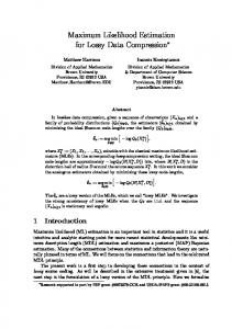
The original data set had no missing data. For that data set, I estimated a least-squares linear regression model with LWAGE as the dependent variable. As predictors, I included FEM, T and their interaction. I used PROC SURVEYREG so that the standard errors would be adjusted for within-person correlation: proc surveyreg data=my.wages; model lwage = fem t fem*t; cluster id; run; Results are shown in Output 1. There is no evidence for an interaction between FEM and T. The main effect of FEM is highly significant, however, as is the main effect of T. Women make about 37% less than men (obtained by calculating 100(exp(-.4556)-1)). For each additional year, there’s about a 10% increase in wages.
Parameter
Estimate
Standard Error
t Value
Pr > |t|
Intercept FEM T FEM*T
6.3399174 -0.4555891 0.0974641 -0.0047193
0.01569031 0.05227259 0.00188545 0.00553191
404.07 -8.72 51.69 -0.85