Handling Missingness when Modelling the Force of Infection from Clustered Seroprevalence Data. Niel Hens∗ , Christel Faes, Marc Aerts, Ziv Shkedy Center for Statistics, Hasselt University, Diepenbeek, Belgium. ∗
[email protected] Koen Mintiens, Veterinary and Agrochemical Research Centre, Ukkel, Belgium Hans Laevens Frank Boelaert European Food Safety Authority, Parma, Italy May 25, 2007
1
Abstract Modelling infectious diseases data is a relatively young research area in which clustering and stratification are key features. It is not unlikely for these data to have missing values. If values are missing completely at random as defined by Little and Rubin (1987), the analysis on the complete cases is valid. However, in practice this assumption is usually not fulfilled. We will show the effect of ignoring missing data in modelling the force of infection of the bovine herpesvirus-1 in Belgian cattle and propose the use of weighted generalized estimating equations with constrained fractional polynomials as a flexible modelling tool.
Keywords: Clustering; Force of Infection; Missing Data; Weighted Generalized Estimating Equations.
2
1
Introduction
Veterinary epidemiology is a research area that deals with the investigation of diseases in animal populations. The seroprevalence survey of the Bovine Herpesvirus-1 (BoHV-1) in Belgian cattle is a study of a transmissible disease in cattle, which is of economic importance and significance to international trade. To facilitate the free trade of cattle, several European countries implemented eradication programs for BoHV-1. BoHV-1 causes infectious bovine rhinotracheitis, an endemic disease. The BoHV-1 seroprevalence (apparent prevalence) in the Belgian cattle population was determined by a large serological survey, conducted from December 1997 to March 1998 (Boelaert et al., 2000; Speybroeck et al., 2003). The sample taken was stratified for province. Within each province, 1% of the total number of herds was sampled. The blood samples, which were taken from all animals in the selected herds, were tested for antibodies against BoHV-1 by using an ELISA-test, specific for the BoHV-1 glycoprotein B (gB). Additional characteristics as gender, type of the herd (dairy, mixed or beef), purchased or homebred and size of the herd were recorded. In total 11,284 cattle were investigated. In Table 1, a complete overview of the variables is given. [Table 1 about here.] A central characteristic of infectious disease dynamics is the transmission of the infection from infectious to susceptible animals. The force of infection (FOI) is the rate of acquisition of the infection for a susceptible host and can be interpreted as the instantaneous probability of getting infected, given that the animal was not infected before. Under the assumptions of life long 3
immunity and that the disease is in a steady state, the prevalence and FOI can be estimated from such seroprevalence data (Grenfell and Anderson, 1985). In Figure 1, the age-specific prevalence of gB-antibodies is displayed. Since animals younger than 6 months typically have high seroprevalence of gB-antibodies because of acquired maternal antibodies and not necessarily due to an infection with BoHV-1, we restricted ourselves to the animals older than 6 months. [Figure 1 about here.] Empirical data in general show that the FOI is age-dependent. Numerous parametric (Grenfell and Anderson, 1985; McCullagh and Nelder, 1989; Grummer-Strawn, 1993; Keiding et al., 1996) and semi-parametric models (Becker, 1989; Jewell and Van Der Laan, 1995; Shkedy et al., 2003, 2006) have been proposed. The BoHV-1 data, like many other infectious diseases data, are complicated and thus statistical modelling has to deal with these complexities. A first important obstacle is the clustering. Indeed, once an infection is introduced in a herd, animals within the same herd have a high chance to get infected too. Thus, individual responses are more homogeneously distributed within herds than in the whole population. In this paper, we utilize generalized estimating equations (GEEs Liang and Zeger, 1986) to account for clustering. GEEs focus on the population mean and recognize the existence of clustering but consider it to be a nuisance characteristic. A second obstacle, of main interest in this paper, is that not all variables are fully observed. From the recorded characteristics, ‘age’, ‘sex’ and ‘gB’ 4
have a small amount of missing values (0.23%, 0.12%, 0.32%, respectively), while the ‘purchase’ variable, indicating whether an animal was homebred or purchased had 2091 missing values (19.00 %). The purchase-missing values were caused by a technical problem while conducting the survey; for animallevel identification, the animals’ working eartag numbers were noted, not their official ones. The eartag numbers have a higher readability, but unfortunately, they were not indexed. Exploratory analyses show that the behaviour of the seroprevalence and FOI is substantially different for purchased compared to homebred animals. Incorporating ‘purchase’ in the analysis is therefore important but introduces difficulties due to missing values. In epidemiological practice, there still is a tendency to analyse the socalled “complete cases”, i.e., those cases which are fully observed, while ignoring the missingness mechanism. If data are missing completely at random (MCAR) as defined by Little and Rubin (1987, Chapter 6), i.e., the missing data mechanism does not depend on either the observed or unobserved data, these complete cases can indeed be analyzed as they are, but even then complete case analysis is non-efficient since one throws away the information still available from the partially observed cases. Moreover, if this MCARassumption is not fulfilled, as is frequently the case in practice, bias can be introduced when merely using the complete cases. Several methods to handle missing data are known. None of them are without limitations. One of them is multiple imputation (Rubin, 1978), where each of the gaps in the data are imputed several times and the analyses of the augmented data sets are then combined. However, in data with a mix of continuous and discrete variables as for the BoHV-1 data, the choice of imputation model is non-trivial. An5
other technique is to weight a subject by the inverse of the probability that it is observed (Zhao and Lipsitz, 1992). In this way subjects unlikely to be observed gain more weight. This can be seen as an implicit imputation of missing values. Both techniques are valid under the MAR-assumption (missing at random), meaning that the missingness mechanism does not depend on unobserved values but possibly on observed values (Little and Rubin, 1987). In this paper, focus is on the effects of missingness when estimating the age-specific FOI for these correlated seroprevalence data. In a first section, we will show how the age-specific FOI is estimated using GEEs to account for the clustering. In a second section, we show that merely using the complete cases leads to inappropriate results and WGEEs can be used to correct for missingness. We are then ready to estimate the FOI while including other risk factors into our model. We end with a general discussion in Section 4.
2
Estimating the Age-specific FOI: Accounting for the Clustering Effect
Mathematical modelling of infectious diseases involves describing the flow of individuals from different infection states within the population (Anderson and May, 1991). Those mathematical models consist of a set of differential equations which aim to describe the flow of individuals from one stage to another. In this paper, we assume the disease is irreversible, meaning that immunity is assumed to be lifelong. We further assume that the mortality caused by the infection is negligible and can be ignored. Under these assumptions the partial differential equation describing the change in the susceptible
6
fraction at age a and time t is given by: ∂ ∂ q(a, t) + q(a, t) = −λ(a, t)q(a, t), ∂a ∂t
(1)
where q(a, t) is the fraction of susceptible individuals at age a and time t. Here λ(a, t) is the rate at which susceptibles become infected and is called the FOI, i.e., the rate at which the host moves from the susceptible to the infected class. We refer to Anderson and May (1991) for more details. The FOI typically is a function of age and time. Estimating the force of infection as a function of age and time is hard since adequate data are mostly not available. Under the assumption of endemic equilibrium also referred to as the steady state assumption it is possible to derive the FOI from serological data. The steady state assumption says that the infectious disease can be sustained in a population without the need for external inputs, i.e. while assuming birth and death rates to be equal, an infected animal infects exactly one other animal. The validity of the steady state assumption can not be verified for a single cross-sectional serological sample since age and time are confounded but turns out to be a helpful starting point in studying the dynamics of an infectious disease as BoHV-1. Let us first derive the FOI in case of a generalized linear model assuming that the disease is in a steady state, i.e., time independent. Let π(a) be the probability to be infected before age a. In general, the seroprevalence π(a) is modelled as π(a) = g −1(η(a)) = δ(η(a)),
(2)
where η(a) is the linear predictor and g is a link function. If it is assumed that the disease is in a steady state, then the age-dependent FOI, λ(a), can 7
be modelled according to equation (Anderson and May, 1991): d q(a) = −λ(a)q(a), da
(3)
with q(a) = 1 − π(a) and so λ(a) =
π ′ (a) . 1 − π(a)
(4)
When, e.g., a logit link is considered, the FOI can be expressed as: λ(a) = η ′ (a)
eη(a) . 1 + eη(a)
(5)
A first step in determining the age-specific FOI for the BoHV-1 data is to model the seroprevalence while dealing with the clustering. There exist several ways to deal with clustering (Aerts et al., 2002). Ignoring the clustering by modelling the seroprevalence using a logistic regression typically leaves the consistency of point estimation intact, but the same is not true for measures of precision. Note that this result is only true when clustersize is uninformative, i.e. not related to the outcome of interest. The issue of dealing with an informative clustersize is covered later in this paragraph and in the discussion. In case of a ‘positive’ clustering effect (i.e., animals within a herd are more alike than between herds), then ignoring this aspect of the data will lead to overestimation of the precision and underestimation of standard errors and lengths of confidence intervals. Both GEEs and random-effects models can be used to deal with clustering. In this paper, we will use the GEE approach and we refer to Faes et al. (2006) for the random-effects approach. Denote Y i = (Yi1 , . . . , Yini )T , the vector of measurements on the i-th cluster and µi = (µi1 , . . . , µini )T , the corresponding vector of means. Let Vi denote the covariance matrix of Y i . 8
Let the vector of explanatory variables for the j-th unit in the i-th cluster be denoted by X ij = (xij1 , . . . , xijp )T and denote g(µij ) = xTij β, where g is the link function. The GEE approach of Liang and Zeger (1986) for estimating the p × 1 vector of regression parameters β is based on solving: S(β, φ; R) =
K X ∂µ i=1
i
∂β
Vi −1 (Y i − µi (β)) = 0.
(6)
Using GEEs, correlated binary data are modelled using the same link function and linear predictor setup (systematic component) as in the independence case (logistic regression). The random component is described by the same variance functions as in the independence case, but the covariance structure of the correlated measurements must also be modelled. This is done by means of a working correlation matrix. The working correlation matrix is usually unknown and must be estimated. It is estimated in the iterative fitting process using the current value of the parameter vector β. Several correlation structures can be specified (Liang and Zeger, 1986). An attractive point of the GEE approach is that it yields a consistent estimator of β even when the working correlation matrix is misspecified (Liang and Zeger, 1986), again when clustersize is uninformative. It has been shown, that in case of a working independence model, which is often convenient, ˆ mostly is relatively efficient (Zeger et al., 1988; McDonald, 1993). But β even if it were not, a more honest estimate of the variability is obtained. Throughout this paper, an independent working correlation will be used. In some situations, like for the BoHV-1 data, the cluster size is related with the outcome of interest. Indeed, animals from larger herds have a 9
higher probability to get infected and thus a larger seroprevalence due to a higher contact rate with other animals (Figure 1). When dealing with an informative cluster size, interest can either go out to the probability of infection of a randomly sampled unit from all units for which no additional adjustment to the analysis has to be made, or, to the probability of infection of a randomly sampled unit from a randomly selected cluster. For the latter situation, Williamson et al. (2003) proposed to weight each animal in a cluster with the inverse of its cluster size to obtain equal weight for all clusters. In this paper, we focus on the first situation while considering the effect of herdsize on the seroprevalence, since veterinarians and animal health policy makers are more interested in inference on the probability to be infected and related force of infection of an arbitrary animal from the full animal population (because they are less interested in interpretations in terms of herds as hierarchical units of the population). We will briefly come back to the second situation in the discussion of this paper. In a parametric model, the relationship between a response variable and several explanatory variables can be expressed in different ways, subject to different assumptions. Using fractional polynomials in the linear predictor part of (2) provides flexibility while attaining the advantages of using a parametric model (Royston and Altman, 1994). For a given degree m a fractional polynomial of age looks like ηm (a; β, p) =
m X
βi Hi (a),
(7)
i=0
where β = (β0 , . . . , βm ) is the vector of regression parameters, p = (p1 , . . . , pm ) a vector of powers p1 ≤ . . . ≤ pm , which are positive or neg10
ative integers or fractions and Hi (x) is a transformation given by p if 0 6= pi 6= pi−1 ai log(a) ifpi = 0 Hi (a) = Hi−1 (a) × log a if pi = pi−1
(8)
with p0 ≡ 0 and H0 ≡ 1. Royston and Altman (1994) argue that polynomials with degree higher than m = 2 are rarely required in practice. The powers themselves are taken from {−2, −1, −0.5, 0, 0.5, 2, . . . , max(3, m)} as proposed by Royston and Altman (1994). The use of splines could offer a fully nonparametric alternative to the use of fractional polynomials. However, the combination of GEEs and (monotone) splines is computationally hard and deals with other issues like, e.g., knot and bandwidth selection. An appealing feature of fractional polynomials is that they, as a parametric tool, offer a wide range of flexible functional forms and that they include the conventional polynomials, often used in practice (Shkedy et al., 2006; Faes et al., 2003). The FOI as a function of age cannot be negative and thus the age-specific ˆ is therefore subject prevalence has to be monotone increasing. Determining β to constraints which depend on the functional relationship with age. We used the ‘Constrained Optimization’-module in Gauss 6.0. The procedure uses a sequential quadratic programming method in combination with the Newton Raphson procedure. In an initial stage, the Broyden-Fletcher-GoldfarbShanno procedure (Shanno, 1985) was used to obtain starting values for the Newton Raphson procedure. Let us now model the seroprevalence using a systematic component of the form g(π) = φ(a) + βherdsize, 11
(9)
where g is a link function, φ is a function of age and herdsize is added to the model to deal with the informative cluster size. Using a logit link and a fractional polynomial of degree 2, we can rewrite model (9) as logit(P (gB = 1)) = β0 + β1 agep1 + β2 agep2 + β3 herdsize.
(10)
The appropriate powers of the fractional polynomial were determined by minimizing Akaike’s Information Criterion. Since we only focus on degree 2 fractional polynomials this corresponds with the deviance criterion used by Royston and Altman (1994). [Table 2 about here.] [Figure 2 about here.] The upper part of Table 2 shows the selected powers, parameters and standard errors. There is a positive effect of herdsize on the seroprevalence and the components of the fractional polynomial counteract. Taking into account the clustering effect has a substantial impact, as can be seen from the differences between the empirical standard errors, i.e., clustering is taken into account, and the model-based standard errors, i.e., ignoring the clustering. The solid curves in Figure 2 show the age-specific seroprevalence (left panel) and FOI (right panel) for herdsizes 15, 45, 80 and 120, representing small, medium, large and very large herds, respectively. There is a clear increase in seroprevalence with age and the FOI reaches a maximum at the ages 1.91, 1.86, 1.80 and 1.73, respectively. This decrease in the age of maximal FOI for an increasing herdsize, shows that the disease spreads faster in larger herds.
12
For all analyses, we omit those cases with missing ‘age’, ‘gb’ and ‘sex’, since this corresponds to only 0.5% of all animals and ignoring them has a negligible impact on the analysis. However, omitting those animals with missing ‘purchase’ from the analyses not only leads to inefficiency but could, depending on the nature of the missing data process, introduce considerable bias (Zhao et al., 1996). In the next section, and before incorporating ‘purchase’ and other variables in the model, we investigate the underlying missingness process.
3
Handling Missingness when Modelling the FOI for the BoHV-1 Study
3.1
Missing data in the BoHV-1 Data
From the 11, 284 records, 2148 records have at least one missing value in response and covariates. For 26 cows (0.26%) age was missing, 14 records (0.12%) did not have gender recorded and the antibody level was missing 36 times (0.32%). The only remaining variable was ‘purchase’ with a substantial amount of missingness since it was not recorded 2091 times (19%). Therefore, for the remainder of this paper observations with one or more missing values for ‘age’, ‘sex’, and ‘gB’ are ignored. Define Rij , an indicator variable which takes the value 1 if, for the j-th animal of the i-th herd, ‘purchase’ is observed and 0 otherwise. To asses the influence of the different variables on the missingness of ‘purchase’, we use a generalized additive model as proposed by Wood (2000); Wood and Augustin (2002); Wood (2004). Starting from the generalized additive model (11), we apply the 3-step method proposed by Wood and 13
Augustin (2002) to drop terms: logit(P (R = 1)) = β0 + fc1 (herdtype) + fc2 (gB) + fc3 (sex) + fc4 (province) + fs1 (age) + fs2 (herdsize) + fs3 (densanim) + fs4 (densherd). (11) fci (·) denotes a main effect of a categorical variable and fsi (·) denotes a smooth function. For this model no term could be dropped. Since the response ‘gB’ has a significant effect on the missingness process, a complete case analysis would indeed result in bias (Zhao et al., 1996). Based on these results, we can show the effect of ignoring missing data (animals for which purchase is missing) when modelling the FOI using model (10). For that purpose, we again consider model (10). We compare the analysis based on the complete cases, i.e., cases for which the ‘purchase’variable is observed with the analysis based on the available cases, i.e., cases for which ‘purchase’ is allowed to be unobserved and show that a weighted analysis on the complete cases can be used to correct for missing ‘purchase’values. The animal-specific weight is the inverse of the estimated probability (see (11)).
3.2
The Effect Of Ignoring Missing Values
When using ‘weighted (generalized) estimating equations’ (Zhao and Lipsitz, 1992; Robins et al., 1994; Zhao et al., 1996), each contribution of a case is weighted with the inverse of the probability that this case is observed. In this way cases, with a low probability to be observed, gain more influence in the analysis and thus represent the missing values resulting in an implicit imputation of missing values. 14
The weighted version of the GEE (6) is given by Sw (β, φ, R) =
K X ∂µ i=1
i
∂β
Vi −1 Wi (Y i − µi (β)) = 0,
(12)
where Wi is a ni × ni diagonal matrix with elements wij equal to the inverse probability for the j-th observed unit in the i-th cluster to be observed, i = 1, . . . , K; j = 1, . . . , ni . These probabilities are preferably estimated semi-parametrically as in (11). If one of these probabilities is estimated to be extremely low, the corresponding animal would receive an excessively large weight. Moreover the size of the herd to which the animal belongs would correspondingly blow up to an unacceptable size. Therefore, as recommended by Little (2004), the estimated weights should, if necessary, be standardized to sum to the total sample size. In our clustered data situation, it has to be checked whether the sum of the estimated weights within a herd approaches the corresponding total herdsize. This was checked in all analyses but no problems were encountered. When dealing with missing data, not only estimation but also the selection of an appropriate model among a set of candidate models based on the complete cases leads to unreliable results. There exist several model selection criteria for GEEs (e.g., AIC, BIC and QIC). Hens et al. (2006) proposed to use weighted model selection criteria for incomplete data. Here, the weights are the same inverse selection probabilities. This again in analogy with the inverse probability weighting used by, e.g., Zhao and Lipsitz (1992); Robins et al. (1994); Zhao et al. (1996). The weighted AIC-criterion was used to select the appropriate powers of the fractional polynomial of age when per15
forming the weighted analysis. In Table 2, the selected powers, parameters and standard errors (columns 1 and 3) for three different methods can be found. The first method corresponds to the GEE-model of Section 2 where all available cases (AC) were used, the second method is based on the complete cases (CC) and the third method uses a WGEE on the complete cases (WCC). The results in this table are difficult to compare since the different methods selected different fractional polynomials. But, in Figure 2, the long and short dashed lines show the resulting seroprevalence and FOI curves corresponding to the use of CC and WCC, respectively. The fits show, especially on the scale of the FOI, that using WCC succeeds in restoring what is observed when using AC and therefore provides correct inferences compared to using CC, especially for larger herdsizes. All methods show a positive effect of herdsize on the seroprevalence and FOI. As pointed out before, there is often interest in the age at which the maximal FOI is reached, agemax . In Table 3 age c max is shown for four herdsizes
15, 45, 80 and 120, representing small, to large-sized farms. For all estimation methods, age c max decreases as herdsize increases. However, using CC, agemax
is severely overestimated with 10 to 17 months compared to age c max based
on AC, while the use of WCC gives a slight underestimation of agemax with about 2.5 months. [Table 3 about here.] These results again show that a beneficial effect of the WCC approach and that using CC can lead to substantial bias.
16
3.3
Including Other Covariates When Estimating The FOI
Until now, we looked at a model of the form (9). Additionally, one can account for heterogeneity related to other covariates by considering g(π) = φ(a) + βherdsize + Xγ.
(13)
Here X denotes the design matrix corresponding to those covariates. Let us consider an additive model consisting of a fractional polynomial of degree 2 for age, herdsize as before, but now including all other variables as main effects. Selecting the appropriate submodel and powers of the degree 2 fractional polynomial of age was done by using the (weighted) AIC-criterion. Deletion of variables stops when the (weighted) AIC-value reaches a minimum. The presented analyses are based on both CC and WCC to show the impact of ignoring missing observations. For both models herdtype was deleted and all other variables were retained. The summary of the final models using (weighted) GEEs; i.e., powers, estimates, empirical and model-based standard errors with corresponding p-values, is given in Table 4. [Table 4 about here.] While there is a clear difference between the empirical and model-based standard errors, reflecting the clustering in the data, this has little impact on the significance (α-level 0.05) of the different covariates. From these analyses one can conclude that purchased animals have a higher seroprevalence than homebred animals. An increasing herdsize, increasing animal density and 17
decreasing herd density give an increase in the seroprevalence. The apparent contradictive effect of animal density and herd density on the seroprevalence has been observed before (Boelaert et al., 2005) and a possible explanation is that low herd density points at regions where family and amateur farms are located, while a high density refers to regions of professional farms. The latter farms are thought to be more aware of the potential danger of infectious diseases. The FOI λ(a) as given in (5) can be denoted as λ(a) = η ′ (a)π(a), i.e. the product of the derivative of the linear predictor w.r.t. age and the seroprevalence. For a model of the form (13) with design matrix X, this turns to φ′ (a)π(a, X) and as a consequence the ratio of FOIs over covariate values can be rewritten as a proportional odds, e.g., for gender: λ(bulls) π(bulls) = . λ(cows) π(cows)
(14)
Bulls have a higher prevalence then cows and thus according to equation (14), bulls have a higher FOI. In veterinary epidemiology, it is known that transport of animals is an important factor for the rate at which the disease spreads and that mostly young animals are more likely to be transported. Therefore, we now look at a model where for both purchased and homebred animals separate fractional polynomials of age are used. Starting from the previous model and including these fractional polynomials, first the animal and then the herd density did no longer contribute significantly to the model. The selected powers, estimates, empirical and model-based standard errors (with corresponding p-values), of the resulting models are given in Table 5. 18
[Table 5 about here.] Whether the animals were purchased or homebred has a substantial influence on the powers chosen for both fractional polynomials. While there is a rather small difference between the use of CC and WCC for homebred animals, there is a considerable one between the two methods for purchased animals. The contributions of the main effects are of the same order as for the additive models except for the province of Brabant where there is a change in sign, although non-significant. From a veterinary point of view, purchased animals are expected to have a higher seroprevalence compared to homebred animals (Boelaert et al., 2005). The interaction model shows that young purchased animals have a higher seroprevalence than young homebred animals, while the seroprevalence for older purchased animals is smaller compared to older homebred animals. Indeed, animals are purchased at a young age and are likely to either be infected or to have recovered from an infection. After introduction into the herd, they can spread the infection to the other animals in the herd, which are mostly homebred. Purchased animals are thus more likely to be infected at a young age in contrast to homebred animals. Secondly, animals in beef herds are slaughtered at young age (18-20 months) and therefore a decline for older ages is caused by the absence of these animals compared to homebred animals.
4
Discussion
The force of infection is one of the primary epidemiological parameters of infectious diseases. A variety of parametric and non-parametric models have 19
been developed to estimate the force of infection from cross-sectional seroprevalence data. It is not unlikely for survey data to have missing values. There is still a great tendency to model incomplete data by simply deleting those subjects with missing values, ignoring the missingness mechanism. This paper addresses the missing data issue in the field of veterinary epidemiology. The analyses on the BoHV-1 data clearly show that inappropriate conclusions can be drawn when the missing data mechanism is ignored. It is shown that an inverse probability weighted analysis (see e.g. Zhao and Lipsitz, 1992) can be used to correct for missing values. This inverse probability weighting was applied to the GEE-approach in combination with a constrained fractional polynomial of age to allow for sufficient flexibility in estimating an age-specific FOI. In this paper, we focussed on modelling the probability of infection for a randomly selected animal from the population of animals while studying the effect of herdsize. If interest would go out to a randomly selected animal from a randomly selected herd, the presented analyses can easily be adapted by assigning herd-specific weights to all animals, where the sum of weights within a herd is standardized to be equal for all herds. Adding covariates like herdsize to the model would then reflect how the seroprevalence of a typical animal from a randomly selected herd would change with different values for this covariate. Furthermore, the inclusion of the inverse probability weighting is easily done by standardisation with respect to the original herdsize instead of the observed herdsize. Modelling the FOI helps understanding the dynamics of the BoHV-1 in20
fection. The main epidemiological conclusion is that purchasing animals and importing them into a herd, facilitates a rapid spread of the infection throughout the herd, resulting in a different behaviour for homebred and purchased animals. It was also observed that larger herds and especially bulls have a higher prevalence and FOI. For a herd of average size, the maximal FOI is observed at 22 months of age. For smaller herds, this increases, while for larger herds it decreases.
Acknowledgements We wish to thank both referees and the editor for valuable remarks leading to an improved presentation. We gratefully acknowledge support from the Fund of Scientific Research (FWO, Research Grant n◦ G039304), the Institute for the Promotion of Innovation by Science and Technology (IWT) in Flanders, Belgium and from the IAP research network nr P5/24 of the Belgian Government (Belgian Science Policy).
References Aerts, M., Geys, H., Molenberghs, G., and Ryan, L. M. (2002), Topics in Modeling of Clustered Data., London: Chapmann and Hall. Anderson, R. M. and May, R. M. (1991), Infectious diseases of humans: dynamic and control., Oxford: Oxford University Press. Becker, N. G. (1989), Analysis of infectious diseases data., London, Chapman and Hall.
21
Boelaert, F., Biront, P., Soumare, B., Dispas, M., Vanopdenbosch, E., Vermeersch, J., Raskin, A., Dufey, J., Berkvens, D., and Kerkhofs, P. (2000), “Prevalence of bovine herpesvirus-1 in the Belgian cattle population.” Preventive Veterinary Medicine, 45, 285–295. Boelaert, F., Speybroeck, N., de Kruif, A., Aerts, M., Burzykowski, T., Molenberghs, G., and Berkvens, D. L. (2005), “Risk factors for bovine herpesvirus-1 seropositivity.” Preventive Veterinary Medicine, 69, 285–295. Faes, C., Geys, H., Aerts, M., and Molenberghs, G. (2003), “On the use of fractional polynomial predictors for quantitative risk assessment in developmental toxicity studies.” Statistical Modelling, 3, 109–126. Faes, C., Hens, N., Aerts, M., Shkedy, Z., Geys, H., Mintiens, K., Laevens, H., and Boelaert, F. (2006), “Population-averaged versus herd-specific force of infection.” Applied Statistics, 55, 595–613. Grenfell, B. T. and Anderson, R. M. (1985), “The estimation of age-related rates of infection from case notifications and serological data.” Journal of Hygiene, 95, 419–36. Grummer-Strawn, L. M. (1993), “Regression analysis of current status data: an application to breast feeding.” Biometrika, 72, 527–537. Hens, N., Aerts, M., and Molenberghs, G. (2006), “Model selection for incomplete and design-based samples.” Statistics in Medicine, 25, 2502–2520. Jewell, N. P. and Van Der Laan, M. (1995), “Generalizations of current status data with applications.” Lifetime data analysis, 1, 101–109. 22
Keiding, N., Begtrup, K., Scheike, T. H., and Hasibeder, G. (1996), “Estimation from current status data in continuous time.” Lifetime Data Analysis, 2, 119–129. Liang, K. and Zeger, S. (1986), “Longitudinal dat analysis using generalized linear models.” Biometrika, 73, 13–22. Little, R. and Rubin, D. (1987), Statistical Analysis with Missing Data., New York.: Wiley. Little, R. J. (2004), “To model or not to model? Competing modes of inference for finite population sampling,” J. Amer. Statist. Assoc., 99, 546–556. McCullagh, P. and Nelder, J. (1989), Generalized Linear Models, Chapman & Hall. McDonald, B. W. (1993), “Estimating logistic regression parameters for bivariate binary data.” Journal of the Royal Statistical Society, Series B, 55, 391–397. Robins, J., Rotnitzky, A., and Zhao, L. (1994), “Estimation of regression coefficients when some regressors are not always observed.” Journal of the American Statistical Association, 89, 846–866. Royston, P. and Altman, D. (1994), “Regression using fractional polynomials of continuous covariates: Parsimonious parametric modelling.” Applied Statistics, 43, 429–467. Shanno, D. F. (1985), “On Broyden-Fletcher-Goldfarb-Shanno method.” Journal of Optimization Theory and Applications, 46, 87–94. 23
Shkedy, Z., Aerts, M., Molenberghs, G., Beutels, P., and Van Damme, P. (2003), “Modelling forces of infection by using monotone local polynomials.” Applied Statistics, 52, 469–485. — (2006), “Modeling age dependent force of infection from prevalence data using fractional polynomials.” Statistics in Medicine, 5:9, 1577–1591. Speybroeck, N., Boelaert, F., Renard, D., Burzykowski, T., Mintiens, K., Molenberghs, G., and Berkvens, D. L. (2003), “Design-based analysis of surveys: a bovine herpesvirus 1 case study.” Epidemiology and Infection, 131, 991–1002. Williamson, J. M., Datta, S., and Satten, G. A. (2003), “Marginal analyses of clusterd data when cluster size is informative .” Biometrics, 59, 36–42. Wood, S. N. (2000), “Modelling and smoothing parameter estimation with multiple quadratic penalties.” Journal of the Royal Statistical Society, Series B, 62, 413–428. — (2004), “Stable and efficient multiple smoothing parameter estimation for generalized additive models.” Journal of the American Statistical Association, 99, 673–686. Wood, S. N. and Augustin, N. H. (2002), “Gams with integrated model selection using penalized regression splines and applications to environmental modelling.” Ecological Modelling, 157, 157–177. Zeger, S. L., Liang, K. Y., and Albert, P. S. (1988), “Models for longitudinal data: A generalized estimating equation approach.” Biometrics, 44, 1049– 1060. 24
Zhao, L. P. and Lipsitz, S. (1992), “Design and analysis of two-stage studies.” Statistics in Medicine, 11, 769–782. Zhao, L. P., Lipsitz, S., and Lew, D. (1996), “Regression analysis with missing covariate data using estimating equations.” Biometrics, 52, 1165–1182.
25
List of Figures 1
2
Seroprevalence plot as a function of age. Each dot represents the age-specific fraction of seropositive animals stratified over small (◦), medium (×) and large (•) herds. . . . . . . . . . . . 27 Age-specific seroprevalence fits together with the age-specific FOI for the available cases (full line), the complete cases (long dashed line) and weighted complete cases (short dashed line) for herdsizes 15, 45, 80 and 120. . . . . . . . . . . . . . . . . . 28
Figure 1: Seroprevalence plot as a function of age. Each dot represents the age-specific fraction of seropositive animals stratified over small (◦), medium (×) and large (•) herds.
Figure 2: Age-specific seroprevalence fits together with the age-specific FOI for the available cases (full line), the complete cases (long dashed line) and weighted complete cases (short dashed line) for herdsizes 15, 45, 80 and 120.
List of Tables 1 2
3 4 5
Overview of the different variables in the BoHV-1 dataset. . GEE parameter estimates, standard errors and corresponding p-values for the three different methods (independent working correlation). . . . . . . . . . . . . . . . . . . . . . . . . . . . Age (in years) where the maximal FOI is reached for herdsize 15, 45, 80 and 120 for the three different methods. . . . . . . Final additive models for the BoHV-1 data: complete cases (upper part) and weighted complete cases (lower part). . . . BoHV-1 data: ‘Purchase (pu) - Homebred (hb)’ - specific fractional polynomial model. . . . . . . . . . . . . . . . . . . . .
. 30
. 31 . 32 . 33 . 34
Table 1: Overview of the different variables in the BoHV-1 dataset. Variable Description gB ELISA-test positive for glycoprotein B, or not herd number of the herd animal number of the animal province province (nine, Brabant Walloon and Flemish Brabant together) herdtype dairy, mixed or beef herdsize size of the herd densanim density of animals in the municipalities (number of cattle/km2 ) densherd density of herds in the municipalities (number of herds/km2 ) age age of the animal (in months) sex gender of the animal purchase purchased or homebred
Table 2: GEE parameter estimates, standard errors and corresponding pvalues for the three different methods (independent working correlation). Parameter Estimate Emp.S.E.(P-value) Mod. S.E.(p-value) Available Cases (-2,-1) Intercept 0.410 0.304(0.177) 0.113(