Handwritten Character Recognition using the Continuos Distance Transformation Joaquim Arlandis Juan-Carlos Perez-Cortes Rafael Llobet Institut Tecnològic d’Informàtica Universitat Politècnica de València Camí de Vera, s/n. 46071, València, Spain e-mail:
[email protected] Abstract In this paper, a feature extraction method for images is presented. It is based on the classical concept of Distance Transformation (DT) from which we develop a generalization: the Continuos Distance Transformation (CDT). Whereas the DT can only be applied to binary images, the CDT can be applied to both binary and gray-scale or color pictures. Furthermore, we define a number of new metrics and dissimilarity measures based on the CDT. Comparative experimental results are also presented for the new measures, using the NIST handwritten characters database. Several experiments using the k-nearest neighbors classification rule are reported, with results that significantly improve the recognition rate of other measures like the Euclidean and some DT-based distances.
1. Introduction Obtaining feature maps from images, where the distance relationships among their pixels are taken into account, is the goal of a well-known technique usually referred to as Distance Transformation or DT [8]. The Distance Transformation is traditionally defined as an operation that transforms a binary digital image consisting of feature and non-feature pixels into a gray-level image (which can also be interpreted as a distance map) where all non-feature pixels have a value corresponding to the distance (any suitable distance function on the plane) to the nearest feature pixel.[2] A large number of works on the Distance Transformation have been published. It was introduced by Rosenfeld and Pfaltz.[8]. Borgefors[1,3] tried to efficiently compute the approximate DT for the Euclidean Distance using masks. More recently, several techniques have been presented achieving a fast and exact Euclidean DT, e.g., Huang et al.[10], who used a technique based on decomposed grayscale morphological operators, and Breu et al.[13], who developed some algorithms to compute the Euclidean
DT in linear time using the Voronoi diagram. Other authors like Kovács and Guerrieri[5] studied the L1 or city-block distance among pixels, and suggested reducing the dimension of a DT map, given the strong correlation among its items. The Absolute Weighted Distances, which are a particular case of the Chamfer Distances, are also used in the computation of the DT [7,12]. Brown[4] presented a simple and fast algorithm to obtain the distance map of a binary image using the L∞ or chessboard distance. The Nearest Feature Transform or FT should be mentioned, which differs from the DT in that it stores the coordinate of the nearest feature pixel rather than the distance to this point. Paglieroni[7] developed a unified distance transform algorithm and architecture based on FT. Wang and Bertrand [11] presented a Generalized Distance Transformation for binary images that is not based on the classical point-to-point concept of the DT nor on the classical metric concept, but on recursive morphological operators. Smith et al.[9] provided results of experiments with handwritten characters using the Pixel Distance as a DT-based distance function. Until now, these studies have focused on binary images. Unfortunately, binarization is a necessary step in order to compute the simple Distance Transformation from continuos-valued images, causing a loss of information. The continuos Distance Transformation or CDT is a new contribution to the computation of distance maps from gray-level or color-level images, in order to make use of the whole information content of their original range of representation. We will also present several distance and dissimilarity measures for images, based on the Continuos Distance Transformation. Some results and conclusions of several experiments performed with a k-nearest neighbors classifier using samples of handwritten upper and lower case letters extracted from the NIST Special Database 3 [6] will also be presented. We have tested some of the mentioned measures in order to assess their performance, compared to binary DT measures and the Euclidean Distance.
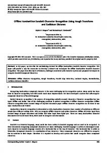
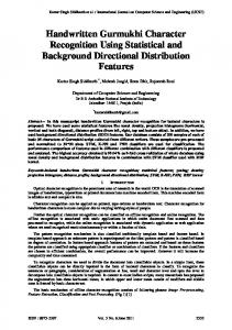
2. The continuos distance transformation Taking the classical definition of Distance Transformation as a basis, we will refer to Distance Map to the Nearest Black Pixel or DTNB if we consider a black pixel as a feature pixel. Therefore, each item of the map DTNB(i,j) holds the distance from pixel (i,j) on the image to the nearest black pixel. Note that this value can be interpreted as the number of fringes expanded from (i,j) until the first fringe holding a black pixel is reached, where each “fringe” is composed by the pixels that are at the same distance of (i,j). In the same way, we can compute a Distance Map to the Nearest White Pixel or DTNW if we consider a white pixel as a feature pixel. Likewise, a Distance Map to the Nearest Pixel of Opposed Color or DTBW will be computed adding the values of the respective matrices representing DTNB and DTNW (see Figure 1). 1 1 1 1 1 1 1
0 0 0 0 0 0 0
0 1 1 0 1 1 1
0 1 1 0 1 2 2
0 1 1 0 1 2 3
0 0 0 0 1 2 3
1 1 1 1 1 2 3
1 1 1 1 1 1 1
1 1 1 1 1 1 1
1 1 1 1 1 2 2
1 1 1 1 1 2 3
1 1 1 2 2 2 3
1 1 1 2 3 3 3
2 2 2 2 3 4 4
Figure 1. Left: DT NB values of an image using L∞ distance. Right: DT BW values of an image using L∞ distance. If we look at a DTNB (Figure 1) or DTNW map, we will note that locations containing zeros mark the presence of feature pixels on the image. The remaining points on the map provide additional information from the original image. In this sense, the DTBW map presents a drawback: it does not provide full information about the original color of the pixels. According to the nature of the image to be analyzed, the DTNB map will be more descriptive if it is applied to images having white background and black foreground, e.g. characters. Conversely, the DTNW map will be more suitable in the opposed case. Finally, the DTBW will be suitable when the binary map distribution is heterogeneous or unknown. Obviously, for many reasons, establishing a parallelism between a distance map of binary images and one of gray-scale images is not trivial. In the first place, the opposing color of a gray value is not well defined, and then, in gray-scale images the distance to the nearest black or white pixel may be meaningless. In order to get a valid generalization of the DTNW for an image whose pixel values are defined in the gray-scale domain [0..MaxBright], we will make a
distance map “to whites”. We will replace the “white pixel” concept by the “maximum bright value” and actions as “find the nearest white pixel” by “accumulate a maximum bright value on an expanding neighborhood”. Moreover, now we will consider that the value of an item on the continuos distance map is a function of the pixel value itself as well as of the number of fringes expanded until an accumulated bright value reaches a threshold according to a certain criteria of bright value accumulation, which is applied to the pixels belonging to each fringe analyzed. So, we substitute the concept of “distance to the nearest white pixel” by the new concept of “distance from a pixel to the limit of their minimum area of brightness saturation”. This approach involves the definition of the next concepts: Minimum Area of Saturation (MAS) and “distance to the limit of MAS”. Since the technique proposed computes continuos distance maps of continuos-valued images (gray or any color space), we call it Continuos Distance Transformation or CDT, of which the traditional DT is a particular case. Two types of CDT-based maps can be defined: Continuos Distance Map to Brightness Saturation or CDTB and Continuos Distance Map to Darkness Saturation or CDTD depending if a maximum value of bright intensity or a maximum value of reverse bright intensity is accumulated, respectively. Both maps provide distinct information about a point and its surrounding area. In [14,15], detailed descriptions of these concepts are presented.
3. Dissimilarity measures based on the CDT: the generalized pixel distances Several distance and dissimilarity measures based on the Continuos Distance Transformation can be used to take advantage of the full possibilities of the representation obtained. For example, metrics as the L-distances between CDT maps can be computed in order to measure image dissimilarities. More complex measures give higher performances. Some of them are generalizations of well-know measures based on the binary Distance Transformation. The Generalized Fringe Distances (based on the Fringe Distance measure enounced by Brown[4]) and the Generalized Pixel Distances (based on the Pixel distance[9]) are well defined and will be presented in this section. The Pixel Distance [9] or PD is a measure of dissimilarity for binary images based on the following concept: two binary images are similar if each pixel (i,j) has the same color on both or, otherwise, there is some pixel having the opposed color in its close neighborhood. Taking into account that the DTBW map holds the distance of a pixel to its closest pixel of opposed color, the expression that computes the Pixel Distance is the following:
Let X, Y be two binary images, PD ( X , Y ) =
∑
∑
i =1.. High j =1..Wide
(X (i , j ) ⊕ Y (i , j ) ) *
(DTBW X (i, j ) + DTBW Y (i, j ) )
An extension of the concept of the Pixel Distance to the continuos-valued domain is now presented. The Generalized Pixel Distances family or GPDn computes the similarity of two continuos-valued images as follows: two images are more similar if the values of a pixel (i,j) are coincident or, otherwise, their respective neighborhoods are similar. Taking into account that both CDTB and CDTD maps reflect the neighborhood of an image, the expression that computes a GPDn distance between two continuos-valued images X, Y defined in the scale [0. MaxBright] is the following: Let X, Y be two continuos-valued images defined in the scale [0..MaxBright], GPDn( X , Y ) =
(
∑
X (i , j ) − Y (i , j )
∑
i =1..High j =1..Wide
CDTB X (i, j ) − CDTB Y (i, j )
n
*
MaxBright +
CDTD X (i, j ) − CDTD Y (i, j )
n
and were tested: upper-case, lower-case letters and digits. All the characters were previously normalized to fill the entire image, keeping the original aspect ratio. To obtain a usable representation of the character images in a low dimensional space, resampling and normalizing procedures are traditionally used. These techniques generate gray-level images that keep most of the original information stored in the full-scale images and, together with the extended distance measures presented, give rise to clearly better results in comparison with binary DT and euclidean distance (ED). In a first phase, Special Database 3 was split into a training set and a validation set. The SD7 was reserved for a second phase and was used only as test set, where the training set included the previous validation set (i.e. the whole SD3 was used for training and SD7 for test). Writers were not shared among the sets. The results are given as recognition percentages at 0%-rejection rate. In all cases, the L∞ or chessboard metric on the plane was used for computing the CDT distance maps.
)
ED
GPD3
Rec. rate
GPD5
0,92 0,91
The weight of the neighborhood in the former expression can be tuned by the exponent n. Notice that, according to above expression, if two points are equal in both images, their difference is 0 and the influence of the CDT maps on the distance will be null. It should be remarked that the binary PD is a particular case of any of the GPDn distances when applied to binary images. There is no direct relation between CDTB and CDTD maps, and then it is reasonable to take into account both of them. This feature makes the GPDn measures able to characterize in a suitable way the dissimilarities between images, mainly when their distribution of brightness is unknown.
0,9 0,89 0,88 0,87 8
10
12
ED
16 22 26 32 Square grid size
GPD3
36
40
Rec. rate
GPD5
0,97 0,96 0,95 0,94
4. Experiments
0,93
The experiments consisted of exhaustive classification tests using the k-NN rule with some distance measures presented in this work. The popular NIST Special Databases 3 and 7 (SD3 and SD7, the last originally known as Test Data 1 or TD1) [6] were used. They are composed of 128x128 pixel segmented binary images of handwritten characters. SD3’s 2,100 writers were American Census field workers, and SD7 was collected among 500 high school student, being very different from the former (some authors refer to SD7 as “hard test” to distinguish it from an “easier test” constituted by splitting SD3 into training and test sets). Three character sets were extracted from the databases
0,92 6
8
10
12 16 22 26 Square grid size
32
36
40
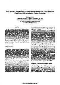
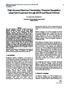
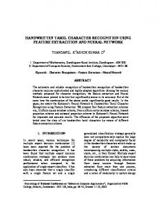
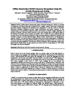
Figure 2. Results of the validation phase for lower-case and upper-case letters, respectively In the validation phase, we tried to determine the optimal parameters that influence the performance of the CDT, namely, the size of the grid and the number of fringe expansions allowed (MaxFringe). We selected the GPD3 and GPD5 measures as well as the ED.
Characters were downsampled to multiple resolutions in order to determine the best ones. In Figure 2, the results are shown for resolutions of 8, 10, 12, 16, 22, 26, 32, 36 and 40 pixels squared. Values of k in [1..10] were tested, and the best one is shown (typically 3, 4, 6 and 8). The values of MaxFringe tested were in [2..max(heigth,width)/2]. Notice the higher performance of the CDT-based measures compared to the Euclidean Distance. The resolutions of 16x16, 22x22 and 26x26 were selected for the test phase experiments. The tests on lower-case and upper-case letters were intended to compare the GPD3 and GPD5 measures, based on the continuos valued transformation, with the binary Pixel Distance (PD) using the classical DT. In Table 1, the higher performance of the classification obtained using CDT-based features is apparent. This confirms that the binarization process after the subsampling involves an important loss of information. Table 1. Results for lower-case and upper-case letters.
16x16 22x22 26x26
LOWER-CASE Training size=45301 Test size= 11999 PD GPD3 GPD5 81.87 85.83 86.16 83.34 86.12 86.07 83.22 86.15 86.22
UPPER-CASE Training size= 44951 Test size= 11938 PD GPD3 GPD5 87.94 92.69 93.04 89.92 93.02 92.81 89.66 93.09 93.20
Finally, the validation and test results for digits are presented. in Table 2. The recognition rates for the different measures are more similar than in the previous case, due to the lower dificulty of the task and the use of larger databases. Table 2. Results for digits. SD3 SD7 Training size=200221 Training size=223124 Validation size= 22903 Validation size= 58646 ED GPD3 GPD5 ED GPD3 GPD5 10x10 99.14 — — 94.76 — — 16x16 — 99.31 99.28 — 95.91 95.89
5
CONCLUSIONS
We have presented the use of the Continuos Distance Transformation as a new feature extraction method for handwritten character recognition. It is a generalization of the classical concept of Distance Transformation that allows the computation of distance transformations to both binary and gray-scale or color pictures. As a consequence, the binarization process, which causes a loss of information, can be avoided. The DT can be seen
as a particular case of CDT. Some CDT-based distances and dissimilarity measures have been tested as well. The experimental analysis with handwritten letters reports that higher recognition rates have been attained using gray-scale than binary image formats and CDT-based measures have better performance than ED and binary DT-based measures.
6. References [1] G. Borgefors, “Distance transformations in arbitrary dimensions”, Computer Vision, Graphics and Image Processing , 1984, vol. 27, pp. 321-345. [2] G. Borgefors, “A new distance transformation approximating the euclidean distance”, Proc. Int’l Joint Conf. Pattern Recognition, 1986, pp. 336-338. [3] G. Borgefors, “Distance transformations in digital images”, Computer Vision, Graphics and Image Processing 34, 1986, pp. 344-371. [4] R.L. Brown, “The fringe distance measure”, IEEE Transactions on Systems Man and Cybernetics 24(1), 1994. [5] Zs.M. Kovács and R. Guerrieri, “Computer recognition of handwritten characters using the distance transform”, Electronic Letters 28(19), 1992, pp. 1825-1827. [6] R.A. Wilkinson, J. Geist, S. Janet, P. Grother, R. Burges, R. Creecy, B. Hammond, J. Hull, N. Larsen, T. Vogl and C. Wilson, First Census Optical Character Recognition System Conference, National Institute of Standards and Techology (NIST), 1992. [7] D.W.Paglieroni, “A unified distance transform algorithm and archietecture”, Machine Vision and Applic. 5, 1992, pp.47-55. [8] A. Rosenfeld and J.L. Pfaltz, “Sequential Operations in digital picture processing”, Assoc.Comput. March 13 1966. [9] S.J. Smith, M.O. Bourgoin, K. Sims and H.L. Voorhees, “Handwritten character classification using nearest neighbor in large database”, IEEE Transactions on Pattern Analysis and Machine Intelligence 16(9), 1994, pp. 915-919. [10] C.T. Huang and O.R. Mitchell, “An euclidean distance transform using grayscale morphology decomposition”, IEEE Transactions on Pattern Analysis and Machine Intelligence 16(4), 1994, pp. 443-448. [11] X. Wang and G. Bertrand, “Some sequential algorithms for a generalized distance transform based on Minkowski operations”, IEEE Transactions on Pattern Analysis and Machine Intelligence 14(11), 1992, pp. 1114-1121. [12] H.G. Barrow, J.M. Tanenbaum, R.C. Bolles and H.C. Wolf, “Parametric correspondence and chamfer matching: two new techniques for image matching”, Proc. 5th Int. Joint Conference on Artificial Intelligence, 1977, pp. 659-663. [13] H. Breu, J. Gil, D. Kirkpatrick and M. Werman, “Linear time euclidean distance transform algorithms”, IEEE Transactions on Pattern Analysis and Machine Intelligence 17(5), 1995, pp. 529-533. [14] J. Arlandis and J.C. Perez-Cortes, “The continuos distance transformation: a generalization of distance transformation for continous-valued images”, Proceedings of the VIII SNRFAI 1, Bilbao, Spain, 1999, pp. 195-202. [15] J. Arlandis and J.C. Perez-Cortes, “The continuos distance transformation: a generalization of distance transformation for continous-valued images”, Pattern Recognition and Applications , IOSPress, Amsterdam, 2000.