Hard X-Ray Detection and Timing of Accretion-Powered ... - CiteSeerX

Space Radiation Laboratory Publication SRL 96-01

Hard X-Ray Detection and Timing of Accretion-Powered Pulsars with BATSE Thesis by Deepto Chakrabarty In Partial Ful llment of the Requirements for the Degree of Doctor of Philosophy

California Institute of Technology Pasadena, California 1996 (Submitted December 21, 1995)

ii

And this is my Quest, To follow that star, No matter how hopeless, No matter how far... |Joe Darion, The Man of La Mancha (1965)

c

1996 Deepto Chakrabarty All rights reserved The pagination of this double-sided printing diers slightly from that of the ocial single-sided version on le with the Institute.

iii

Acknowledgements Unwept, unhonor'd, and unsung. |Sir Walter Scott (1805)

I am indebted to Tom Prince for being an outstanding advisor and mentor. I am full of admiration for the various attributes which constitute his style of doing science: the skill at choosing important problems to study, the rigorous approach to posing and de ning the boundaries of these problems, the elegant and ambitious tools aggressively applied to solve them, the polished communication of the results, and the cool, professional detachment with which unexpected diculties are confronted, appraised, and overcome. The sheer number of projects he is able to pursue successfully is mind-boggling. I very much appreciate Tom's indulgence in allowing me to pursue a wide variety of projects myself, and also his admonitions to maintain sucient focus to make important contributions rather than merely skim the surface. I am also grateful to Lars Bildsten, who has played a very large role in my development as an astrophysicist. His unerring ability to a reduce a problem to its basic physics after a few minutes at the blackboard, the clarity of his explanations and insights, and his seemingly endless and encyclopedic knowledge of astronomy and astrophysics have been an education in how to think about problems and what questions to ask. His practical insights and candid advice on the daily trials of doing science and his cheerful willingness to always look at \just one more cool plot" were also greatly appreciated. In working on the BATSE Pulsar Key Project, I have been fortunate to collaborate with some outstanding researchers, especially John Grunsfeld and my fellow graduate student Danny Koh here at Caltech, and Mark Finger of the BATSE instrument team at NASA/MSFC. I owe special thanks to John, who trained me in the day-to-day business of high-energy astrophysics and oversaw much of my work during my rst two years here. His enthusiasm, ambition, and tenacity were a lesson by example. I am glad that I overlapped with the recent arrival of Brian Vaughan, and with the even more recent arrival of Rob Nelson; they were both welcome additions to the Caltech eort. Thanks to Jerry Fishman, Bob Wilson and the entire BATSE group at MSFC for many useful discussions throughout my thesis work, and especially during my visits to Huntsville; and to Jerry Fishman in

iv particular for acting as agency sponsor for a NASA graduate fellowship. Special thanks are due to the entire BATSE instrument team, which has had the dicult task of supporting BATSE, its operations, and its guest investigators, while also pursuing a wide range of science topics. One of the privileges of working in astrophysics at Caltech is the large number of faculty, sta, and postdoctoral scientists on hand to learn from. I happily acknowledge many useful discussions with Stuart Anderson, Lee Armus, Roger Blandford, John Carlstrom, Curt Cutler, Melvyn Davies, Fiona Harrison, Vicky Kaspi, Dong Lai, Rob Nelson, Gerry Neugebauer, Neill Reid, Maarten Schmidt, Tom Soifer, Steve Thorsett, Marten van Kerkwijk, and Brian Vaughan. One of Caltech's most precious resources in astrophysics has been its Astrophysics Library and its librarians, Helen Knudsen and Anne Snyder. Our community has suered a serious loss with Helen's recent retirement. I have been further privileged to work in Caltech's Space Radiation Laboratory. Thanks to Frances Spalding and Louise Sartain at SRL for awlessly navigating me through administrative hurdles; Laura Carriere, Minerva Calderon, and Bruce Sears for working day and night (literally) to keep our computers crunching numbers and exchanging e-mail; and Debby Kubly for doing her best to nd me good mail every day. I have pursued several optical follow-up projects related to my thesis work. These eorts have been both productive and fun, in large part due to my long-time collaborator in much of this work, Paul Roche. Thank you to Malcolm Coe for his hospitality and support during a visit to Southampton work with Paul. Jim McCarthy, Xiaopei Pan, Marshall Cohen, Angela Putney, Ian Thompson, and Bob Hill answered many questions while I was learning to use the instruments at Palomar Observatory, and Skip Staples and Jean Mueller kept things running smoothly during the observations. I am grateful to my old friend Stephen Levine for helping to put together a productive visit to the Observatorio Astronomico Nacional 2.1-m telescope on an isolated mountain top in San Pedro Martir, Baja California, and I thank Luis Aguilar and the UNAM Insituto de Astronoma in Ensenada for covering my expenses during this trip. I am also grateful for a generous travel grant and observing time allocation from the Cerro Tololo Inter-American Observatory in Chile for thesis-related work. It is a pleasure to thank Andy Layden, Ramon Galvez, Patricio Ugarte, Arlo Landolt, and Bruce Margon for helpful assistance, discussions, and guidance during my visit to CTIO. Thanks also to Paul Eskridge and Stefanie Wachter for taking some nder images for me on other CTIO telescopes.

v I probably would not have been invited to study at Caltech had it not been for the research opportunities given me by Richard Muller at LBL, and I would not have thought to contact Rich about a job after nishing at MIT had it not been suggested by my old friend Don Alvarez. Thanks to both of them for helping to get me here. Since then, my 5.2 years at Caltech have been made much easier by the wonderful friends I've met here. From the very rst day on campus, no physics graduate student at Caltech can fail to appreciate the care with which Donna Driscoll looks after us. Getting through the rst year courses would have much more unpleasant without the weekly late-night get-togethers in the LIGO conference room with Ruth Brain, Aaron Gillespie, James Larkin, Torrey Lyons, Sima Setayeshgar, Selmer Wong, and our other classmates. For close friendships forged through work, lunch, coee, dinner, spirited arguments, idle chatting, and evenings of random cosmopolitanism (kudos to Charlene Reichert for coining this apt term), I would especially like to thank Paul Ray, Bi Heindl, Fiona Harrison, Lars Bildsten, Steve Thorsett, Andrea Ghez, Tom LaTourrette, Alycia Weinberger, David Hogg, Vicky Kaspi, Dominic Benford, and Alan Wiseman. Some of these people left Caltech before me, while others will remain after I leave, but they are all a large part of what I will remember when I think back to these years. I have been lucky to share a spacious and comfortable apartment with my friend Robert Knop. I thank Robert for his patience with me and for endless hours of shared zaniness involving musical revues, physics, theatre, neural nets, chamber music, waltz orchestras, pizza, ice cream, the Oph object, Unix, and various incarnations of Star Trek. I also thank him in advance for teaching me to solder. A large fraction of my waking hours have been spent at the lab, and these hours have been made more fun and interesting by my oce-mates: David Palmer, Je Hammond, Tim Shippert, Alycia Weinberger, Stinson Gibner, Bi Heindl, Daniel Williams, Yu Cao, Song Wang, and Stephane Corbel. I thank Shirley Marneus, Delores Bing, and Allen Gross for my providing me with opportunities to indulge my interests in the arts. In these activities, I have had the pleasure of working with some ne musicians, especially Tom LaTourrette, Diana Lorden, Jamie Schlessman, Russ Litch eld, Peter Hofstee, Jerome Claverie, Ari Kaplan, Missy Richmond, and Elizabeth Boer. Life in graduate school is a lengthy and trying eort, especially in the bizarre land that is Los Angeles, and the connections to my family and old friends back in civilized places like New York, Boston, and the Bay Area were necessary to get through it. All

vi the visits and talks with people like Beth Multer, Larry Arnold, Corinne Wayshak, Patrick Beard, and Tim Sasseen were essential to maintaining my sanity. For the last two years, getting to know my very special and sweet friend Susan Elia has brought me great joy. For more than half a lifetime, I have been able to depend on one of my oldest and best friends, Nina Sonenberg. But I am most grateful for the lifelong and unconditional love, support, and encouragement always oered by my parents and my sister, even when they did not understand what I was doing or why. It is a pleasure to acknowledge support from a National Aeronautics and Space Administration Graduate Student Research Program fellowship, under grant NGT-51184. I also thank the National Science Foundation for generous travel support which allowed me to attend two NATO Advanced Study Institutes: \The Gamma-Ray Sky with Compton GRO and SIGMA" in Les Houches, France, in January 1994; and \Evolutionary Processes in Binary Stars" in Cambridge, England, in July 1995. The research in this thesis was supported in part by the NASA Compton Observatory Guest Observer Program, under grant NAG 5-1458; and by the NASA Long-Term Space Astrophysics Program, under grant NAGW-4517.

vii

Hard X-Ray Detection and Timing of Accretion-Powered Pulsars with BATSE Deepto Chakrabarty

California Institute of Technology

Abstract The BATSE all-sky monitor on the Compton Gamma Ray Observatory is a superb tool for the study of accretion-powered pulsars. In the rst part of this thesis, I describe its capabilities for hard X-ray observations above 20 keV, present techniques for timing analysis of the BATSE data, and discuss general statistical issues for the detection of pulsed periodic signals in both the time and frequency domains. BATSE's 1-day pulsed sensitivity in the 20{60 keV range is 15 mCrab for pulse periods 2 s< Ppulse 12 10 G. Close to the neutron star, the eld disrupts the accretion ow, attaching matter onto the eld lines and channeling it onto the magnetic poles. The resulting accretion luminosity thus emanates from two restricted \hot spots" on the neutron star. The pulsed emission is thought to arise from a misalignment of the magnetic axis and the spin axis which causes the hot spots to sweep across our line of sight at the spin period. The pulse pro les of X-ray pulsars tend to be fairly broad and sinusoidal, particularly above 10 keV. This is especially true in comparison to the sharp, narrow pro les typically observed in the radio pulsars. The pulse shapes can be roughly described as either single-peaked or doublepeaked (although some have complex substructure, particularly at low energies). This is

REFERENCES

13

believed to re ect whether the emission from one or both magnetic poles is crossing our line of sight. Some accreting pulsars (e.g., Vela X-1, GX 301{2) which are single peaked at soft X-ray energies become double peaked in BATSE's energy range.

References Adams, W. S. 1915. The spectrum of the companion of Sirius. Pub. Astron. Soc. Paci c, 27, 236. Adams, W. S. 1925. The relativity displacement of the spectral lines of the companion of Sirius. Proc. Natl. Acad. Sci. (USA), 11, 382. Baade, W. & Zwicky, F. 1934. Supernovae and cosmic rays. Phys. Rev., 45, 138. Chadwick, J. 1932. The existence of a neutron. Proc. R. Soc. London A, 136, 692. Chandrasekhar, S. 1931. The maximum mass of ideal white dwarfs. Astrophys. J., 74, 81. Cominsky, L., Roberts, M., & Finger, M. H. 1994. An April 1991 outburst from 4U 0115+63 observed by BATSE. In Second Compton Symposium, ed. C. E. Fichtel, N. Gehrels, & J. P. Norris (New York: AIP), 294. Cook87 Cook, M. C. & Page, C. G. 1987. The X-ray properties of 3A 1907+09. Mon. Not. R. Astron. Soc., 225, 381. Corbet, R. H. D. 1986. The three types of high-mass X-ray pulsator. Mon. Not. R. Astron. Soc., 220, 1047. Corbet, R. H. D., Woo, J. W., & Nagase, F. 1993. The orbit and pulse period of X1538{522 from Ginga observations. Astron. & Astrophys., 276, 52. Davidson, K. & Ostriker, J. P. 1973. Neutron star accretion in a stellar wind: model for a pulsed X-ray source. Astrophys. J., 179, 585. Deeter, J. E. et al. 1987. Pulse timing study of Vela X-1 based on Hakucho and Tenma data: 1980{1984. Astron. J., 93, 877. Deeter, J. E. et al. 1991. Decrease in the orbital period of Hercules X-1. Astrophys. J., 383, 324. Dirac, P. A. M. 1926. On the theory of quantum mechanics. Proc. R. Soc. London A, 112, 661. Finger, M. H. 1993. Personal communication. Finger, M. H. 1995. Personal communication. Finger, M. H. et al. 1993. BATSE observations of Cen X-3. In Compton Gamma Ray Observatory, ed. M. Friedlander et al. (New York: AIP), 386. Finger, M. H. et al. 1994. Hard X-ray observations of A0535+262. In Evolution of X-Ray Binaries, ed. S. S. Holt & C. S. Day (New York: AIP Press), 459. Finger, M. H., Wilson, R. B., & Chakrabarty, D. 1996. Reappearance of the X-ray binary pulsar 2S 1417{624. Astron. & Astrophys., in press. Finger, M. H., Wilson, R. B., & Fishman, G. J. 1994. Observations of accretion torques in Cen X-3. In Second Compton Symposium, ed. C. E. Fichtel, N. Gehrels, & J. P. Norris (New York: AIP Press), 304.

14

CHAPTER 1. ACCRETION-POWERED PULSARS AND BATSE

Finger, M. H., Wilson, R. B., & Harmon, B. A. 1996. Quasi-periodic oscillations during a giant outburst of A0535+26. Astrophys. J., in press. Fowler, R. H. 1926. On dense matter. Mon. Not. R. Astron. Soc., 87, 114. Frank, J., King, A., & Raine, D. 1992. Accretion Power in Astrophysics (Cambridge: Cambridge U. Press). Gamow, G. 1937. Structure of Atomic Nuclei and Nuclear Transformations (Oxford: Clarendon). Giacconi, R., Gursky, H., Paolini, F. R., & Rossi, B. B. 1962. Evidence for X-rays from sources outside the solar system. Phys. Rev. Lett., 9, 439. Giacconi, R., Gursky, H., Kellogg, E., Schreier, E., & Tananbaum, H. 1971. Discovery of periodic X-ray pulsations in Centaurus X-3 from Uhuru. Asrophys. J., 167, L67. Gold, T. 1968. Rotating neutron stars as the origin of the pulsating radio sources. Nature, 218, 731. Harrison, B. K., Thorne, K. S., Wakano, M., & Wheeler, J. A. 1965. Gravitation Theory and Gravitational Collapse (Chicago: U. Chicago Press). Hellier, C. 1994. 4U 0142+614 and RX J0146.9+6121. IAU Circ., No. 5994. Hewish, A., Bell, S. J., Pilkington, J. D. H., Scott, P. F., & Collins, R. A. 1968. Observation of a rapidly pulsating radio source. Nature, 217, 709. Hughes, J. P. 1994. A new transient pulsar in the Small Magellanic Cloud with an unusual X-ray spectrum. Astrophys. J., 427, L25. Israel, G. L., Mereghetti, S., & Stella, L. 1994. The discovery of 8.7 second pulsations from the ultrasoft X-ray source 4U 0142+61. Astrophys. J., 433, L25. Israel, G. L., Stella, L., Angelini, L., White, N. E., & Giommi, P. 1995. HD 49798 and 2E 0050.1{ 7247. IAU Circ., No. 6277. Kelley, R. L., Rappaport, S., & Ayasli, S. 1983. Discovery of 9.3-s X-ray pulsations from 2S 1553{542 and a determination of the orbit. Astrophys. J., 274, 765. Koh, T. et al. 1995. GRO J1750{27 and GRO J1735{27. IAU Circ., No. 6222. Koh, T. et al. 1996. BATSE observations of the accreting X-ray pulsar GX 301{2. Astrophys. J., in preparation. Koyama, K. et al. 1989. Are there many Be star binary X-ray pulsars in the Galactic ridge? Pub. Astron. Soc. Japan, 41, 483. Lamb, F. K., Pethick, C. J., & Pines, D. 1973. A model for compact X-ray sources: accretion by rotating magnetic stars. Astrophys. J., 184, 271. Landau, L. D. 1932. On the theory of stars. Physikalische Zeitschrift der Sowjetunion, 1, 285. Landau, L. D. 1938. Origin of stellar energy. Nature, 141, 333. Levine, A. et al. 1991. LMC X-4: Ginga observations and search for orbital period changes. Astrophys. J., 381, 101. Levine, A. et al. 1993. Discovery of orbital decay in SMC X-1. Astrophys. J., 410, 328. Lewin, W. H. G. 1994. Three decades of X-ray astronomy from the point of view of a biased observer. In Evolution of X-Ray Binaries, ed. S. S. Holt & C. S. Day (New York: AIP Press), 3.

REFERENCES

15

Makishima, K. et al. 1984. Discovery of a 437.5-s pulsation from 4U 1907+09. Pub. Astron. Soc. Japan, 36, 679. Makishima, K. et al. 1987. Spectra and pulse period of the binary X-ray pulsar 4U 1538{52. Astrophys. J., 314, 619. Nagase, F. 1989. Accretion-powered X-ray pulsars. Pub. Astron. Soc. Japan, 41, 1. Oppenheimer, J. R. & Serber, R. 1938. On the stability of stellar neutron cores. Phys. Rev., 54, 540. Oppenheimer, J. R. & Volko, G. M. 1939. On massive neutron cores. Phys. Rev., 55, 374. Pacini, F. 1967. Energy emission from a neutron star. Nature, 216, 567. Pringle, J. E. & Rees, M. J. 1972. Accretion disc models for compact X-ray sources. Astron. & Astrophys., 21, 1. Rappaport, S. et al. 1978. Orbital elements of 4U 0115+63 and the nature of the hard X-ray transients. Astrophys. J., 224, L1. Rubin, B. C. et al. 1994. BATSE observations of 4U 1538{52: a 530 second pulsar. In Evolution of X-Ray Binaries, ed. S. S. Holt & C. S. Day (New York: AIP Press), 455. Sandage, A. R. et al. 1966. On the optical identi cation of Sco X-1. Astrophys. J., 146, 316. Sato, N. et al. 1986. Orbital elements of the binary X-ray pulsar GX 301{2. Astrophys. J., 304, 241. Schmidtke, P. C., Cowley, A. P., McGrath, T. K., & Anderson, A. L. 1995. Discovery of an X-ray pulsar in the LMC. Pub. Astron. Soc. Paci c, 107, 450. Schwentker, O. 1994. Evidence for a low-luminosity X-ray pulsar associated with a supernova remnant. Astron. & Astrophys., 286, L47. Schreier, E., Levinson, R., Gursky, H., Kellogg, E., Tananbaum, H., & Giacconi, R. 1972. Evidence for the binary nature of Centaurus X-3 from Uhuru X-ray observations. Astrophys. J., 172, L79. Shapiro, S. L. & Teukolsky, S. A. 1983. Black Holes, White Dwarfs, and Neutron Stars (New York: Wiley). Shklovsky, I. S. 1967. On the nature of the source of X-ray emission of Sco XR-1. Astrophys. J., 148, L1. Stella, L. et al. 1985. The discovery of 4.4 second X-ray pulsations from the rapidly variable X-ray transient V0332+53. Astrophys. J., 288, L45. Stollberg, M. H. et al. 1994. Recent observations of EXO 2030+375 with BATSE. In Evolution of X-Ray Binaries, ed. S. S. Holt & C. S. Day (New York: AIP Press), 255. Taylor, J. H., Manchester, R. N., & Lyne, A. G. 1993. Catalog of 558 pulsars. Astrophys. J. Suppl., 88, 529. Waters, L. B. F. M. & van Kerkwijk, M. H. 1989. The relation between orbital and spin periods in massive X-ray binaries. Astron. & Astrophys., 223, 196. White, N. E., Nagase, F., & Parmar, A. N. 1995. The properties of X-ray binaries. In X-Ray Binaries, ed. W. H. G. Lewin, J. van Paradijs, & E. P. J. van den Heuvel (Cambridge: Cambridge U. Press), 1.

16

CHAPTER 1. ACCRETION-POWERED PULSARS AND BATSE

White, N. E., Swank, J. H., & Holt, S. S. 1983. Accretion powered X-ray pulsars. Astrophys. J., 270, 711. Wilson, C. A. et al. GRO J2058+42. IAU Circ., No. 6238. Wilson, C. A., Finger, M. H., Harmon, B. A., Scott, D. M., Wilson, R. B., Bildsten, L., Chakrabarty, D., & Prince, T. A. 1996. BATSE observations and orbital determination of the X-ray pulsar GS 0834{430. Astrophys. J., submitted. Wilson, R. B. et al. 1994a. Discovery of the hard X-ray pulsar GRO J1008{57 by BATSE. In Evolution of X-Ray Binaries, ed. S. S. Holt & C. S. Day (New York: AIP Press), 451. Wilson, R. B. et al. 1994b. Observation of a correlation between main-on intensity and spin behavior in Her X-1. In Evolution of X-Ray Binaries, ed. S. S. Holt & C. S. Day (New York: AIP Press), 475.

17

Chapter 2 Acquisition and Reduction of BATSE Data There is likely to be a still undetected but entirely measurable ux of -rays bearing astronomical information of the highest interest. |Philip Morrison (1958) It is important to understand your background at least as well as you understand your signal. |Thomas A. Prince (1992)

2.1 The Compton Gamma Ray Observatory The Compton Gamma Ray Observatory (GRO; Figure 2.1) was launched from NASA Kennedy Space Center, Cape Canaveral, Florida, on the space shuttle Atlantis (STS37) on 1991 April 5. The 15900 kg satellite, which is the heaviest unmanned scienti c payload ever deployed in space, is in a 400 km orbit inclined 28.5 with respect to Earth's equator. Compton is the second of four planned elements of the NASA Great Observatories program1 . It carries four instruments which span the 20 keV{30 GeV gamma-ray spectrum. The Burst and Transient Source Experiment (BATSE; Fishman et al. 1989) provides a nearly continuous all-sky monitor of the gamma-ray sky in the 20 keV{1.8 MeV range using uncollimated NaI scintillators. The Oriented Scintillation Spectroscopy Experiment (OSSE; Johnson et al. 1993) measures gamma-ray spectra in the 50 keV{10 MeV range using collimated NaI/CsI scintillators. The Compton Telescope (COMPTEL; Schonfelder et 1 The

others are the Hubble Space Telescope (HST), launched in 1990; the Advanced X-ray Astrophysics Facility (AXAF; see Weisskopf 1988), scheduled for launch in 1998; and the Space Infrared Telescope Facility (SIRTF; see Fazio & Eisenhardt 1990), scheduled for launch in 2001.

18

CHAPTER 2. ACQUISITION AND REDUCTION OF BATSE DATA +Z AXIS (YAW) COMPTEL

BATSE 6 EGRET

BATSE 4

OSSE BATSE 2

+X AXIS (ROLL) BATSE 0

MAGNETIC TORQUERS

HIGH-GAIN ANTENNA

+Y AXIS (PITCH)

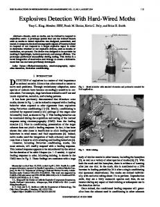
Figure 2.1: The Compton Gamma Ray Observatory. The 8 BATSE detector modules are situated on the corners of the spacecraft's main body. Modules 0, 2, 4, and 6 are visible in this diagram.

al. 1993) provides imaging observations in the 1{30 MeV range using a combination liquid scintillator/NaI scintillator detector. The Energetic Gamma Ray Experiment Telescope (EGRET; Thompson et al. 1993) provides imaging in the 20 MeV{30 GeV range using a spark chamber detector. A recent review of Compton Observatory science was given by Shrader & Gehrels (1995).

2.2 The Burst and Transient Source Experiment BATSE, whose instrumentation is described in detail by Fishman et al. (1989) and Horack (1991), consists of eight identical uncollimated detector modules arranged on the corners of the Compton spacecraft. Each detector module contains three detectors: a large-area detector (LAD), a smaller spectroscopy detector (SD), and a charged-particle

2.2. THE BURST AND TRANSIENT SOURCE EXPERIMENT

19

Figure 2.2: A BATSE detector module. The investigations in this thesis all employ data from the large area detectors.

detector (CPD). Our pulsar studies deal entirely with data from the LADs, each of which contains a NaI(Tl) scintillation crystal 1.27 cm thick and 50.8 cm in diameter, viewed in a light collection housing by three 12.7 cm diameter photomultiplier tubes. The LADs are shielded in front by a 1 mm aluminum window and by the CPDs, which are 0.63 cm thick polystyrene scintillators operated in anticoincidence with the LADs to provide a charged particle veto. The LADs have an eective energy range of 20 keV{1.8 MeV. Below 30 keV, the sensitivity is severely attenuated by the aluminum and plastic shielding. The rear of each detector module is protected by a passive lead-tin shield which is opaque to photons below 300 keV. Scintillation pulses from the LADs are processed in two parallel paths: a fast (1.5 s deadtime), four-channel discriminator circuit and a slower (2.5{25 s deadtime, depending on photon energy) multi-channel pulse height analyzer. The nominal energies for

20

CHAPTER 2. ACQUISITION AND REDUCTION OF BATSE DATA Table 2.1. Energy Channels in BATSE DISCLA and CONT Data Channel

Energy Range (keV)

Background,Rate (count s 1 )

DISCLA 1 DISCLA 2 DISCLA 3 DISCLA 4

20{60 60{110 110{320 >320

1500 1200 1000 700

CONT 0 CONT 1 CONT 2 CONT 3 CONT 4 CONT 5 CONT 6 CONT 7 CONT 8 CONT 9 CONT 10 CONT 11 CONT 12 CONT 13 CONT 14 CONT 15

20{24 24{33 33{42 42{55 55{74 74{99 99{124 124{165 165{232 232{318 318{426 426{590 590{745 745{1103 1103{1828 >1828

250 450 500 500 500 450 300 300 300 200 130 130 50 80 80 200

NOTE: These channel boundaries are approximate, and are averaged over the eight detectors. Each detector has slightly dierent edges. The CONT edges are programmable; the displayed values are typical.

the upper three discriminators are 60 keV, 110 keV, and 320 keV. The lower level discriminators are programmable and are currently set to approximately 20 keV. The pulse height analyzer constructs 128-channel high energy resolution (HER) spectra from the LAD data. The mapping between HER channel number and energy is calibrated separately for each detector using ground test data and ight observations of the Crab Nebula (Pendleton et al. 1994). The calibration is maintained during ight by an automatic correction scheme which adjusts the detector gain to keep the 511 keV line feature in the gamma-ray background aligned in the correct HER channel. The BATSE data types fall into four categories.

2.3. DETECTOR RESPONSE

21

Background data. These consist of the background DISCLA and CONT products,

which are available continuously. The 4-channel LAD discriminator rates (DISCLA data) are sampled every 1.024 s. The 128-channel high energy resolution (HER) spectra are mapped into medium-resolution 16-channel spectra every 2.048 s, called continuous (CONT) data. The mapping of HER channels to CONT channels is programmable, and is occasionally changed temporarily to optimize the tradeo between energy and time resolutions for a particular science investigation. The typical energy channel boundaries for the DISCLA and CONT data are given in Table 2.1. Housekeeping data. The HKG product contains information on the spacecraft orientation as well as its geocentric position at 2.048 s intervals. These positions are accurate to 6 km (3). The QUAL product contains diagnostic information on data quality, identifying intervals which should be excluded from data analysis due to telemetry errors, spacecraft reorientations, etc. We also use the QUAL information to exclude intervals containing gamma-ray bursts from pulsar timing analysis. Scheduled data. There are several data products which can be specially scheduled and provide high time or energy resolution. Several pulsar modes are available which can provide time resolution as short 16 ms for limited observation intervals. Burst trigger data. A variety of special data products are activated with high time and energy resolution when triggered by on-board identi cation of a gamma-ray burst in the BATSE LAD data stream. These data products are not relevant for pulsar studies.

2.3 Detector Response The eective area for the LADs at normal incidence as a function of energy is shown in Figure 2.3. The solid curve represents the eective area for any interaction in the detector, while the dashed curve shows the eective area for full energy deposition. Despite the fact that the photoelectric absorption cross-section of NaI increases steeply at low energies, the eective area curve below 100 keV is dropping rapidly. This is due to the attenuation of low energy photons by the aluminum window and the CPD. Figure 2.4 shows the angular response of the LADs to a monochromatic photon beam at various energies, computed using the detector response matrices of Pendleton et

22

CHAPTER 2. ACQUISITION AND REDUCTION OF BATSE DATA

Figure 2.3: Eective area of a BATSE large area detector at normal incidence. The solid curve denotes the total response of the detector, including interactions where the incident photon energy is only partially deposited. The dashed curve denotes the response for full energy deposition in the detector. The feature near 30 keV is due to the iodine K edge. Adapted from Fishman et al. (1989).

al. (1995). The dominant eect governing this response is the projected detector area along the line of sight to the source, which varies as cos (where is the viewing angle between the detector normal and the source). However, while the response to 100 keV photons is approximately cos , the response at energies both above and below 100 keV diverge from this for dierent reasons. At higher energies, the photon attenuation length in NaI is comparable to the thickness of the crystal, so any interactions tend to occur deep in the crystal. The decrease in projected geometric area with increasing is partially oset by the increase in path length through the detector, both of which have a cos dependence. This results in a relatively at angular response for > 50 at high energies. The response does not fall to zero at 90 incidence due to the nite thickness of the crystal.

2.3. DETECTOR RESPONSE

23

Figure 2.4: Angular response of a BATSE large area detector to photons of various energies. For comparison, a cos response is indicated by the dotted curve. The secondary maximum in the 20 keV response at large angles is due to a gap in the detector support structure at the edge of the LADs. Computed using the detector response matrices of Pendleton et al. (1995).

At low energies, the attenuation length is very short and the interactions occur near the surface of the crystal, making its eective thickness irrelevant. However, the path length through the shielding in this case increases with , and the resulting attenuation of

ux incident on the LAD causes the response to fall more steeply than cos . The secondary maximum in the large-angle response for low energies is due to the geometry of the support structure at the edge of the LADs. There is a gap through which low energy photons in that restricted angular range can reach the NaI crystal without passing through most of the shielding. This feature is poorly calibrated and may not be azimuthally symmetric. A consequence of the variation of angular response with energy is that the integrated angular response to a source is dependent upon its intrinsic energy spectrum. Typical

24


Figure 2.5: BATSE LAD angular response to an incident photon power-law spectrum dN=dE / E , , for = 2 and = 5. For comparison, cos response (dotted line) and cos2 response (dashed line) are also shown.

accreting pulsar spectra in the 20{100 keV range can be modeled by a photon power-law of the form dN=dE / E , with photon index 2 < < 5. Figure 2.5 shows the angular response to a 20{75 keV photon power law spectrum for the extreme cases of = 2 and

= 5. For comparison, cos and cos2 responses are also plotted. We see that the predicted response falls o more quickly than cos because the large number of incident low-energy photons dominate despite the attenuation by the shield. As expected, this eect is more pronounced for the steeper power-law index, where the proportion of incident high-energy photons is even lower. By comparison, Brock et al. (1991) predict an approximately cos response for gamma-ray bursts, which they model as having a 50{300 keV photon power law with a low-energy cuto. In general, the integrated response varies approximately as cos for small angles ( < 25 ), independent of photon index. At larger angles, cos2 is a

2.4. OPTIMAL COMBINATION OF DETECTORS

25

more conservative general assumption if the source spectrum is unknown.

2.4 Optimal Combination of Detectors Because of the octahedral arrangement of the BATSE detector planes, an astrophysical source is visible in four BATSE detectors during any given spacecraft pointing. (The spacecraft is typically reoriented at two-week intervals.) We consider here how to optimally combine data from these four detectors in order to maximize the signal-to-noise ratio. For the purposes of this calculation, we will consider background-limited observations of a constant source and will assume that the background noise is constant, isotropic, and governed by Poisson statistics. Then, the signal-to-noise ratio is given by P S (2.1) SNR = p wP(i ) r(i ) ; B w(i ) where S is the source count rate in a single detector at normal incidence, B is the background count rate in each detector, i is the source viewing angle for ith detector, r() is the angular response function of the detector, and w() is the detector weighting function which we are trying to optimize. It is more convenient to work with the signal-to-noise relative to that of a single detector at normal incidence, P (2.2) relative SNR = p[wP(i )= max(w)] r(i ) : [w(i )= max(w)] The optimal choice of weighting function w() will depend on the form of the detector angular response r(). However, we showed in the previous section that the form of r() depends upon the intrinsic energy spectrum of the source. In what follows, we will assume that the source of interest is an accreting pulsar with a 20{75 keV photon power law spectrum and that the angular response function as r() = cos2 . For a given spacecraft orientation, BATSE is more sensitive to some areas of the sky than others. The highest sensitivity is at the eight points in the sky which lie on the BATSE detector normals (i.e., the direction vector for normal incidence), while the lowest sensitivity is at six points in the sky which lie equidistant from the four incident detector normals. The weighting function for summing detectors which optimizes the tradeo between maximizing signal and minimizing noise, as parametrized in Equation (2.1), depends upon where in the sky the source is relative to the detector normals. For a source lying along one of the detector normals, adding in the data from any of the other three viewing detectors

26


(which each have 70 incidence) with any non-zero weight will reduce sensitivity. On the other hand, the best sensitivity for a source equidistant from the four detector normals is obtained by combining the four detectors with equal weight. Indeed, it is interesting to note that an unweighted combination of the four incident detectors yields uniform sensitivity over the whole sky, under our assumptions. Speci cally, this is a consequence of the assumed cos2 response of the detectors, as we now show. Consider a source at azimuth A and altitude a relative to the spacecraft axes. For de niteness, let us suppose that this source is incident upon detectors 0, 1, 4, and 5. From the altazimuth direction vectors for the corresponding detector normals (see Appendix A), the detector viewing angles are given by cos 0 = p1 (cos A cos a + sin A cos a + sin a) 3 1 cos 1 = p (cos A cos a + sin A cos a , sin a) 3 1 cos 4 = p (, cos A cos a + sin A cos a + sin a) 3 1 cos 5 = p (, cos A cos a + sin A cos a , sin a): 3 Taking w() = 1 for an unweighted sum and inserting into Equation (2.2), we nd that 2 2 2 2 relative SNR = cos 0 + cos 1p+ cos 4 + cos 5 4 2 = 3;

independent of sky position. However, this isotropic response sacri ces the increased sensitivity possible at certain sky locations. We have calculated sensitivity as a function of sky position for weighting functions of the form cosn , with n = 0; 1; 2; 3; 4. The results are shown in Figure 2.6 and summarized in Table 2.2. All the results are quoted relative to the sensitivity of a single detector at normal incidence. The best overall sensitivity is achieved by choosing the detector weighting adaptively based on the altazimuth position of the source. The detector weighting used in all the analyses presented in this thesis was w() = cos2 . An alternative family of weighting schemes is unweighted sums of subsets of the four incident detectors: singles, pairs, triples, and quads. This set of schemes is especially relevant for blind searches, since unweighted combinations can provide good sky coverage and sensitivity without resorting to an inecient grid search. We have calculated the relative


Figure 2.6: Optimal detector weighting for known sky positions. Sky coordinates are shown in the altazimuth system with respect to the spacecraft axes.

27

28


Figure 2.7: Optimal detector combinations for blind searches. Sky coordinates are shown in the altazimuth system with respect to the spacecraft axes.


Table 2.2

Relative sensitivity of various detector weighting schemes Sensitivity Weighting Minimum Maximum Mean 1 0.67 0.67 0.67 cos 0.63 0.93 0.76 cos2 0.60 0.94 0.79 3 cos 0.58 0.96 0.80 cos4 0.56 0.99 0.80 adaptive 0.67 0.99 0.81

Figure 2.8: View directions for the various BATSE detector combinations. Each digit represents the corresponding detector. Sky coordinates are shown in the altazimuth system with respect to the spacecraft axes.

29

30


Table 2.3

Relative sensitivity of various detector combinations Sensitivity Search pattern Minimum Maximum Mean Eciency singles (8) 0.33 1.00 0.75 9.4% pairs (12) 0.47 0.94 0.81 6.8% triples (24) 0.58 0.77 0.74 3.1% quads (6) 0.67 0.67 0.67 11.0% singles+pairs+quads (26) 0.67 1.00 0.85 3.2% all combinations (50) 0.67 1.00 0.85 1.7% singles+pairs (20) 0.47 1.00 0.84 4.2% sensitivity of the various unweighted combination schemes, along with the overall eciency (de ned as the mean sensitivity divided by the number of possible combinations). The results are shown in Figure 2.7 and summarized in Table 2.3. For each sky position in a given scheme, the most sensitive combination was chosen; the possibility of correlating information from overlapping combinations was not considered. The altazimuth sky positions for the various detector combinations is shown in Figure 2.8. In the context of blind searches, we see again that the exclusive use of quads (i.e., unweighted 4-detector sums) provides uniform sky coverage at the expense of some loss in sensitivity. This might be desirable for certain kinds of investigations. The use of unweighted singles+pairs+quads gives better overall sensitivity than the adaptive cosn weighting scheme. Adaptive selection of this unweighted scheme (or else the addition of unweighted pairs to the adaptive cosn scheme) is the overall best weighting choice.

2.5 Earth Occultation Viewed from an altitude of 400 km, the Earth covers about 33% of the sky and subtends an angle of 140 . Over the course of a spacecraft orbit at this altitude, 93% of the sky (corresponding to angles > 20 from the orbital poles) is subject to occultation. The Compton orbital plane is inclined 28.5 with respect to the Earth's equator, and the orbital poles precess around the Earth's polar axis with a 53 d period due to perturbations by the Earth's equatorial bulge (see Figure 2.12). The entire sky is subject to Earth occultation over at least some portion of the precession period. Bright sources subject to occultation will

2.5. EARTH OCCULTATION

31

Figure 2.9: Earth occultation of Cygnus X-1, as observed in the 20{60 keV channel of the BATSE large area detector facing the source. (Figure adapted from Zhang et al. 1994.)

be visible as sharp edges in the BATSE data stream as the source passes behind the Earth's limb and then reemerges (see Figure 2.9); the height of these edges is a direct measure of the total (pulsed+unpulsed) instantaneous ux. By timing these edges, one can localize sources along the arc corresponding to the limb of the Earth across the sky. For a given sky region, the orientation of these limbs rotate over the 53-d Compton orbital precession period, eventually providing source localization within 0:1 , limited by the time resolution of the data and variations in the gamma-ray opacity of the Earth's upper atmosphere (Harmon et al. 1992; Zhang et al. 1994). Fainter sources require averaging of multiple edges; the detection threshold for 1 day of 20{60 keV DISCLA data is 100 mCrab. Knowledge of the occultation times for a given sky direction is important for any BATSE data analysis (pulsed or unpulsed), since the signal-to-noise ratio of an observation can always be improved by discarding data during occultations. For most of the analyses


32

presented in this thesis, occultation times were calculated by assuming the Earth is spherical and modeling its atmosphere as opaque to gamma-rays below an altitude of h = 70 km and transparent above this altitude. A source is occulted when the impact parameter of the line of sight with respect to the Earth is less than R + h. The impact parameter obeys the relation b2 = r2 + s2 + 2r s; (2.3) where b is the impact parameter, r = (x; y; z ) is the geocentric equatorial spacecraft position vector, s = su^ is the line-of-sight vector from the spacecraft to the impact parameter vector, and u^ = (cos cos , cos sin , sin ) is the equatorial direction vector for a source at right ascension and declination . We can compute the impact parameter more accurately by accounting for the Earth's oblateness as follows2 . The surface of an oblate spheroid is given by

r = q(1 , f sin2 )

(2.4)

where q is the equatorial radius, f = (q , c)=q is the attening factor, c is the polar radius, and is the latitude. It is reasonable to assume that atmospheric density is a function of gravitational potential and that the equipotential surfaces are similar oblate spheroids. Given a position vector r = (x; y; z ), the equatorial radius of the equipotential passing through that position is given by 2 q2 = (1 , frsin2 )2 = r2 [1 + 2f sin2 + O(f 2 )] x2 + y2 + z2(1 + 2f ):

(2.5)

We can now de ne an eective impact parameter in terms of

b2e = As2 + Bs + C; with

A = u2x + u2y + u2z (1 + 2f ) B = 2xux + 2yuy + 2zuz (1 + 2f ) C = x2 + y2 + z 2 (1 + 2f ): 2 Based

on a suggestion by W. A. Wheaton of JPL.

(2.6)

2.6. DETECTOR BACKGROUND

33

Minimizing with respect to s, we nd that the eective impact parameter is 2 be = C , 4BA

!1=2

:

(2.7)

We can achieve additional accuracy by abandoning the step-function model for the occultation edges and instead calculating the relative atmospheric transmission along the line of sight. We will assume an exponential atmosphere with density q , b e (q) = (be ) exp , h ;

(2.8)

where h is the scale height of the atmosphere. The optical depth of the atmosphere along this line of sight is Z1 = 2 (q)ds; (2.9) 0

where is the mass attenuation coecient of air and we have assumed that the spacecraft is well outside the atmosphere. Noting that s = q sin and making a substitution of variables, we have Z =2 = 2be (be ) exp , bhe cos1 , 1 cosd2 : (2.10) 0

Assuming be h, we can eectively make a small angle approximation,

2be (be ) p

Z1 0

!

2 exp ,b2eh d

= (be ) 2be h:

(2.11) (2.12)

The occultation transmission function is then given by e, , which varies monotonically between zero and one over an occultation step. Typical parameter values are h = 6 km, (70 km) = 3 10,3 g cm,3, and = 0:3 cm2 g,1 .

2.6 Detector Background Gamma-ray observations in low Earth orbit must contend with a low instantaneous signal-to-noise ratio due to the high background count rate. A detailed review of the gammaray background for low-Earth orbit instruments in general is given by Dean, Lei, & Knight (1991); a discussion of the background for BATSE in particular is given by Rubin et al. (1996). The typical BATSE background as a function of energy is shown in Figure 2.10. The background count rate in the 20{100 keV range is over two orders of magnitude larger than the count rate for a typical accreting pulsar in BATSE data.

34


Figure 2.10: Typical count spectrum of the background as a function of energy for a BATSE LAD. The count spectrum is fairly at in the 20{40 keV range and is well-described by an E ,1:7 power law above 40 keV. This plot can be used to predict the LAD background rate in an arbitrary energy range.

For pulsar studies, we are mainly interested in energies below 100 keV. In this regime, the dominant background component is diuse cosmic emission. The raw 20{60 keV BATSE LAD count rates for one day of data are shown in Figure 2.11. The quasisinusoidal variations with a 93 min period are due to the spacecraft orbital modulation of sky area visible to the detectors. At these energies, the maximum background occurs when the detector is facing away from Earth, and the minimum occurs when the detector is facing toward Earth. The large gaps in the data occur during passages of the spacecraft through a region of extremely high background known as the South Atlantic magnetic anomaly (SAA; see Tascione 1988). Due to the extremely high ux of trapped charged particles in this region, the detector high voltage is turned o to prevent electrical breakdown damage. Smaller gaps due to brief telemetry errors are also sometimes present. It is instructive to consider the power spectral properties of the BATSE background in the frequency domain. The mean raw background rate in the 20{60 keV DISCLA data is 1500 counts s,1 . A steady, unmodulated photon background of this strength would be a Poisson process and would have a power spectral density of 1500 counts2 s,2 Hz,1 ,


Figure 2.11: Raw DISCLA channel 1 (20{60 keV) count rates from the 8 BATSE LADs on 1994 June 2 (MJD 49505). The data shown are averaged at 50 s intervals. The large o-scale events (e.g., near t = 15000 s) occur at the edges of passages through the South Atlantic magnetic anomaly.

35

36


Figure 2.12: Decay of the Compton spacecraft orbit. (Left panel:) Evolution of the Compton orbital period. (Right panel:) Evolution of the precession period of Compton's ascending node. The discontinuity of both plots near day MJD 49300 is due to the reboost of the Compton spacecraft during that interval.

independent of frequency. However, as is evident in Figure 2.11, the BATSE background is by no means steady and unmodulated. The strong 93 min orbital modulation results in a large excess of power at frequencies near gro 2 10,4 Hz. In addition, the complicated time structure of the SAA gaps and the sharp occultation edges caused by bright astrophysical sources are also modulated at the orbital period, introducing signi cant power at higher harmonics of gro. There are also power contributions at beat frequencies of gro and its harmonics with the Earth's daily rotation period. For analysis of long time series of BATSE data, power contributions at harmonics of the precession frequency of the spacecraft orbit, as well as at beats with these frequencies, are also important. Periodic and secular variations in the spacecraft orbital parameters caused by the tidal perturbations and atmospheric drag (see Figure 2.12) result in a modulation of the relevant families of low-frequency noise peaks in the power spectrum. The complex low-frequency noise contributions to the BATSE background result in a signi cant departure from Poisson statistics in the raw data, especially at long time scales (top curve of Figure 2.13). We can improve our sensitivity to pulsed signals by attempting


37

Figure 2.13: Typical pulse frequency dependence of the BATSE LAD background in the 20{60 keV range. The top curve is for the unprocessed raw data. The middle curve is for the raw data after subtraction of an ad hoc background model. The bottom curve is for the raw data after subtraction of the Rubin et al. (1996) physical background model. The dotted line shows the Poisson noise level expected for the raw count rates. For both versions of the background subtraction, the background uctuations are consistent with the Poisson level on time scales < 100 s. The data shown are for DISCLA channel 1 (20{60 keV) from LAD 0 on 1994 June 2 (MJD 49505). A peak near 0.28 Hz due to the pulsar 4U 0115+63 is visible in the background-subtracted data.

to remove the background contributions. There are two basic approaches to this task: Ad hoc background model. We can construct an ad hoc model for the background by removing impulsive spikes and interpolating over gaps in the raw data and then smoothing. The resulting time series is a good approximation to the orbital background variation, which can be subtracted from the raw data. Any sort of smoothing or averaging will aect low-frequency signals as well as background. To keep track of this explicitly, we perform the smoothing in the frequency domain by multiplying the Fourier transform of the interpolated raw time series by a frequency-dependent (low pass) lter function 8 < 1 1 + cos 2 0 R( ) = : 0

for < 0 for 0 < < Nyq

(2.13)

38

CHAPTER 2. ACQUISITION AND REDUCTION OF BATSE DATA where 0 is the cuto frequency of the low-pass lter and Nyq is the Nyquist frequency of the time series. (For all of the analysis presented in this thesis, 0 = 1:6 10,3 Hz). We then use the inverse Fourier transform of this product as an approximate background model, which we subtract from the raw time series. After this subtraction, we discard the interpolated segments by reintroducing the original gap structure into the background-subtracted time series. The power spectrum of a time series with the ad hoc background model subtracted is shown in the middle curve of Figure 2.13. Most of the noise reduction is from the elimination of broadband \ringing" harmonics introduced by spikes and gaps. We emphasize the explicit side eect of this technique, that real signals with periods > 1=0 640 s are attenuated along with the noise background. Physical background model. Both the BATSE instrument team (Rubin et al. 1996) and investigators at JPL (Skelton et al. 1993) have developed semi-empirical physical models for the known sources of background in the BATSE data. The Rubin et al. (1996) model includes the diuse cosmic gamma-ray background, the atmospheric gamma-ray background caused by cosmic ray interactions, the prompt background due to cosmic ray interactions with material on the spacecraft, the delayed internal background caused by activation of spacecraft material by cosmic rays and trapped particles in the SAA, and occultation edges due to bright astrophysical sources. This technique assumes the presence of periodic behavior at harmonics of the orbital period, so some attenuation of low frequency signal as well is inevitable in the tting process.

For both methods of background subtraction, the noise power is consistent with the Poisson level on time scales < 80 s. However, at longer time scales, a strong noise red-noise component is still present, although at a substantially reduced level compared to the original time series. The physical background model performs somewhat better than the ad hoc model at long time scales, yielding a factor of 3 reduction in the noise power (corresponding to p a factor of 3 improvement in sensitivity at these pulse frequencies).

2.7. SENSITIVITY TO PULSED SIGNALS

39

2.7 Sensitivity to Pulsed Signals 2.7.1 General Principles Astrophysical observations with non-imaging instruments require a way to distinguish source emission from background. The usual approach is to split the observation into two adjacent pointings of equal duration: an on-source interval and an o-source interval, with as much overlap in the background regions as possible. This technique is ineective with BATSE due to its large eld of view and highly variable background. Earth occultation measurements provide the only means to make a background-limited observation of a steady source with BATSE. In this case, the occultation step provides the dierentiation between on-source and o-source within the same pointing. In a similar vein, pulsations also provide a way to distinguish between source and background within the same pointing. However, in this case, only the pulsed component can be measured; the steady component is indistinguishable from the background. All of the observations described in this thesis fall into this last category. To compute the signal-to-noise ratio of pulsed signal in the presence of a background which may depend upon pulsed frequency, it is convenient to work in the frequency domain. For a sinusoidal signal with amplitude a and frequency 0 , the signal strength is p characterized by the root-mean-squared amplitude s = a= 2. The noise is given by q

n = s2 + b2 ( );

(2.14)

where s2 is the variance of the signal strength and b2 is the variance of the background level. For a steady pulsed signal, the signal variance is simply given by Poisson statistics,

a ; s2 = pa = p 2 T 2

(2.15)

where = 1=T is the frequency resolution of the observation, T is the duration of the observation, and the result is independent of 0 . The variance of the background is 2 ( ) = dP = 1 dP ; (2.16) b 0

d

=0

T d

=0

where dP=d is the power spectral density of the background uctuations. Our pulsar observations are in the background-limited regime (b s ), so the signal-to-noise ratio (SNR) is given by 1=2 dP ,1=2 aT SNR = p d : (2.17) 2 =0

40


Figure 2.14: Typical BATSE pulsar detection sensitivity as a function of energy, for 1 day of data. The solid line denotes the count ux density required for a signal-to-noise ratio of 5. For comparison, the expected ux densities for a Crab-like source at 15 mCrab and 100 mCrab are shown by the dotted curves.

It is interesting to compare this to the usual (time-domain) expression for SNR in a background-limited observation, s SNR = s Tb ;

(2.18)

where b is the mean background rate. We can evidently regard dP=d as numerically equivalent to an eective background rate. Indeed, we saw in the previous section that dP=d is numerically identical to the mean BATSE background rate at high frequencies p where Poisson statistics are operative. We also note the factor of 2 reduction in the SNR for a sinusoidally pulsed signal. This is because of the reduced duty cycle of a sinusoid compared to a constant signal. The SNR for a more complicated pulse shape can be computed by superposition of appropriately scaled harmonics. In this case, the background power should be computed separately for each harmonic.

2.7.2 BATSE Sensitivity as a Function of Energy We can use the count spectrum of the background in Figure 2.10 to estimate the energy dependence of BATSE's pulsed source sensitivity. Let us con ne ourselves to pulse periods P < 80 s, so that we can assume Poisson statistics for dP=d . The detection

2.7. SENSITIVITY TO PULSED SIGNALS

41

Figure 2.15: Typical BATSE pulsar detection sensitivity as a function of pulse frequency, for 1 day of 20{60 keV DISCLA data. The upturn above 0.2 Hz is due to the 1.024 s binning of the data. At low frequencies, the physical model-subtracted data is at least a factor of 2 more sensitive than the ad hoc model-subtracted data, which has reduced sensitivity below 1:6 10,3 Hz due to signal attenuation by the digital ltering process. The low-frequency sensitivity shown for the physical model-subtracted data does not take into account the loss of sensitivity caused by \absorption" of signal power in the background- tting process. Data shown are from LAD 0 on 1994 June 2 (MJD 49505).

threshold for SNR=5 in 1 day of data is shown with the solid curve in Figure 2.14. The dotted lines represent the expected count spectrum for sources with spectra similar to the Crab Nebula ( = 2:15) incident photon power-law spectrum, with intensities of 15 mCrab and 100 mCrab. We see that the 15 mCrab source is only detected below below 30 keV, while the 100 mCrab source can be detected well above 100 keV. Actual accreting pulsars tend to have spectral cutos in the 20{40 keV range, with their spectra falling faster than the Crab's above this energy.

2.7.3 BATSE Sensitivity as a Function of Pulse Frequency Since most of our pulsar detection studies are done with the 20{60 keV DISCLA data, it is of particular interest to determine the pulse frequency dependence of BATSE's sensitivity in this energy range. We have used the frequency-dependent noise background measurement in Figure 2.13 to compute the sensitivity achieved in a 1-day observation of a source at normal incidence using background-subtracted data. The results are plotted in

42

CHAPTER 2. ACQUISITION AND REDUCTION OF BATSE DATA Table 2.4. Leap Seconds Date

Starting Epoch

1991 Jan 1 1992 Jul 1 1993 Jul 1 1994 Jul 1 1996 Jan 1

MJD

TAI,UTC (s)

48257.0 48804.0 49169.0 49534.0 50083.0

26.0 27.0 28.0 29.0 30.0

New updates of the leap second schedule can be obtained from the U.S. Naval Observatory via WWW ( le://maia.usno.navy.mil/ser7/tai-utc.dat).

Figure 2.15. BATSE's sensitivity degrades rapidly for pulse frequencies < 0:01 Hz, although the physical model-subtracted data degrade more slowly than the ad hoc model-subtracted data. Above 0.2 Hz, there is a loss of sensitivity due to binning of the data (see x3.2.3). The expected response for high-frequency (aliased) signals is indicated by the dashed line.

2.8 Time Systems and Reference Frames The Compton Observatory orbits Earth and Earth orbits the Sun. Both these eects will introduce periodic advances and delays in the BATSE measurements of astrophysical pulse arrival times, or equivalently periodic Doppler shifts in measurements of pulse frequencies. These eects are removed by transforming to a reference frame at the solar system barycenter which is inertial with respect to the pulsar3. A more subtle correction is necessary as well. Pulsar timing measurements can probe small time variations over long time scales and consequently require extraordinarily careful attention to the terrestrial time standards to which measurements are referred. Indeed, some millisecond radio pulsars have such superb intrinsic temporal stability, and can be timed with such high precision, that they provide an experimental probe of theories of gravity. By contrast, the accreting pulsars studied in this thesis are very noisy clocks. Moreover, their substantially slower rotation periods ease the required timing accuracy of 3 Of course, there will also be a periodic variation due to the binary motion of the pulsar, but this is one of the things we want to measure! Once the pulsar orbital parameters are known, the observations can be further transformed to a frame which is inertial with respect to the center of mass of the pulsar binary, allowing us to probe the rotation history of the neutron star without orbital contamination.

2.8. TIME SYSTEMS AND REFERENCE FRAMES

43

the observations by three orders of magnitude. Still, it is essential to reduce the observations to an inertial, uniform dynamical time system. There are several time scale systems which are relevant to our observations4 . At present, the most precise determination of time available is provided by atomic clocks. International Atomic Time (TAI) is a time scale constructed by averaging a large number of atomic clocks worldwide and provides the basis for the SI second. Coordinated Universal Time (UTC) is the basis of civil timekeeping. It is closely tied to the observationally determined time scale UT1, which is related to the mean apparent motion of the Sun due both to the rotation and the orbit of Earth. Due to irregularities in Earth's rotation, UT1 gradually accumulates discrepancies with respect to TAI. UTC is an arti cial time scale which diers from TAI by an exact integer number of seconds, and is maintained within 0.9 s of UT1 by the intermittent introduction of leap seconds (see Table 2.4). The time system which we want to refer our data to is dynamical time. This theoretical time scale is the independent variable in physical equations of motion. Due to relativistic eects, this time scale depends upon the reference frame in which it is measured. Motion referred to a geocentric reference frame can be expressed in terms of Terrestrial Dynamical Time (TDT), while motion referred to the solar system barycenter is expressed in terms of Barycentric Dynamical Time (TDB). TDT is speci ed with respect to TAI and is currently set as TDT = TAI + 32.184 s (exactly), so that they are identical except for a constant oset. TDB is speci ed with respect to TDT through a relativistic correction for gravitational redshift and time dilation due to the motion of the Earth with respect to the solar system barycenter. For the analyses in this thesis, a more-than-suciently accurate relation (Seidelmann, Guinot, & Doggett 1992) is TDB = TDT + (0:001658 s) sin M + (0:000014 s) sin 2M;

(2.19)

where M , the mean anomaly of Earth, is given by

M = 357:53 + 0:98560028 (MJD , 51544:5):

(2.20)

In pulsar astrophysics, this relativistic correction is called the solar system Einstein delay. In summary, there are a series of corrections which must be applied to the BATSE observation times. BATSE data are recorded with UTC measurement times at the spacecraft. By adding the appropriate number of leap seconds (Table 2.4) and a constant 32.184 s 4 The

discussion that follows draws from Seidelmann, Guinot, & Doggett (1992).

44


oset, we readily obtain TDT at the spacecraft (tGRO ). To obtain TDB at the solar system barycenter (tb ), we can follow Taylor & Weisberg (1989) by writing

tb = tGRO + r c ^s + E + S :

(2.21)

The second term on the right-hand side is the projected light travel time correction from the spacecraft to the barycenter along the line of sight to the pulsar, sometimes called the solar system Romer delay; r is the position vector of Compton with respect to the solar system barycenter, and ^s is the unit vector toward the pulsar. The spacecraft barycentric position is calculated as r = RGRO + r: (2.22) The geocentric spacecraft vector RGRO is recorded in the BATSE housekeeping data (x2.2), and the barycentric vector for the Earth r is computed using the Jet Propulsion Laboratory DE-200 solar system ephemeris (Standish et al. 1992). The third term in Equation (2.21), E , is the solar system Einstein delay given in Equation (2.19). The nal term in Equation (2.21), S , is a relativistic correction for the propagation of the pulsar photons through the gravitational eld of the Sun. This eect, called the solar system Shapiro delay, is of order 5 s and thus utterly negligible for our purposes.

2.9 Standard Analysis Procedure The standard pulsed source analysis consists of the following steps (see Figure 2.16):

Background-subtraction. The four detectors viewing the direction of interest are

conditioned to remove the orbital background. Timing studies using the DISCLA data were background-subtracted using the ad hoc model technique. Spectral studies using the CONT data were processed with the Rubin et al. 1996 background model. Optimal combination of detectors. The four detectors are summed using a cos2 weighting scheme. Mask out bad data and Earth-occulted intervals. Bad time intervals, as indicated by the QUAL le information, are masked out of the summed time series. Intervals during Earth occultation of the direction of interest are also masked out.

2.9. STANDARD ANALYSIS PROCEDURE

Figure 2.16: Standard BATSE analysis sequence. The data shown are for LAD 0 on 1994 June 2 (MJD 49505). The top panel shows the raw time series. The second panel shows the time series after subtraction of the ad hoc background model. The third panel shows the Fourier power spectrum of the ltered time series. The peak near 0.27 Hz is due to 4U 0115+63. The bottom panel shows the power spectrum renormalized by the local noise power. The pulsed signal due to 4U 0115+63 is evident.

45


46

Apply barycenter correction. If the source position is known accurately, then

the data are transformed from UTC times at the spacecraft to an inertial frame in terms of TDB times at the solar system barycenter. If the source position is not well known but the observation is long enough that ignoring the barycenter correction would introduce decoherence eects (see Appendix B), then an approximate source position can be used to apply a rough barycenter correction. Operationally, the barycenter correction consists of ve steps: 1. Measure UTC time at Compton. 2. Add appropriate number of leap seconds to obtain TAI time at Compton. 3. Add 32.184 s to obtain TDT at Compton. 4. Add solar system Einstein delay to obtain TDB at Compton. 5. Add light travel time correction to obtain TDB at barycenter.

All pulsar timing parameters in this thesis are referred to TDB at the solar system barycenter. The time series obtained after the above steps is the basic data set used for our pulsar studies at Caltech.

References Brock, M. N., Meegan, C. A., Roberts, F. E., Fishman, G. J., Wilson, R. B., Paciesas, W. S., & Pendleton, G. N. 1991. Gamma ray burst locations from the Burst and Transient Source Experiment. In Gamma Ray Bursts, ed. W. S. Paciesas & G. J. Fishman (New York: AIP), 383. Dean, A. J., Lei, F., & Knight, P. J. 1991. Background in space-borne low-energy -ray telescopes. Space Sci. Rev., 57, 109. Fazio, G. G. & Eisenhardt, P. 1990. The Space Infrared Telescope Facility (SIRTF). In Observatories in Earth Orbit and Beyond, ed. Y. Kondo (Dordrecht: Kluwer), 193. Fishman, G. J. et al. 1989. BATSE: the Burst and Transient Source Experiment on the Compton Gamma Ray Observatory. In Proc. of the GRO Science Workshop, ed. W. N. Johnson (Greenbelt: NASA/GSFC), 2-39. Harmon, B. A. et al. 1992. Occultation analysis of BATSE data: operational aspects. In Compton Observatory Science Workshop, ed. C. R. Shrader, N. Gehrels, & B. Dennis (Washington: NASA CP-3137), 69. Horack, J. M. 1991. Development of the Burst and Transient Source Experiment (BATSE) (Washington: NASA Reference Publication 1268). Johnson, W. N. et al. 1993. The Oriented Scintillation Spectrometer Experiment: instrument description. Astrophys. J. Suppl., 86, 693.

REFERENCES

47

Pendleton, G. N. et al. 1995. The detector response matrices of the Burst and Transient Source Experiment (BATSE) on the Compton Gamma Ray Observatory. Nucl. Instr. Methods A, 364, 567. Pendleton, G. N., Paciesas, W. S., Briggs, M. S., Harmon, B. A., & Wilson, C. A. 1994. Channel to energy calibration results for the BATSE large area detectors. In Second Compton Symposium, ed. C. E. Fichtel, N. Gehrels, & J. P. Norris (New York: AIP), 749. Rubin, B. C., Lei, F., Fishman, G. J., Finger, M. H., Harmon, B. A., Paciesas, W. S., Pendleton, G. N., & Wilson, R. B. 1996. A model of the gamma-ray background on the BATSE experiment. Astron. & Astrophys. Suppl., in press. Schonfelder, V. et al. 1993. Instrument description and performance of the imaging gamma-ray telescope COMPTEL aboard the Compton Gamma Ray Observatory. Astrophys. J. Suppl., 86, 657. Seidelmann, P. K., Guinot, B., & Doggett, L. E. 1992. Time. In Explanatory Supplement to the Astronomical Almanac, ed. P. K. Seidelmann (Mill Valley: University Science Books), 39. Shrader, C. R. & Gehrels, N. 1995. Recent results from the Compton Gamma Ray Observatory. Pub. Astron. Soc. Paci c, 107, 606. Skelton, R. T., Ling, J. C., Ling, N. F., Radocinski, R., & Wheaton, W. A. 1993. Status of the BATSE enhanced Earth occultation analysis package for studying point sources. In Compton Gamma-Ray Observatory, ed. M. Friedlander, N. Gehrels, & D. J. Macomb (New York: AIP), 1189. Standish, E. M., Newhall, X. X., Williams, J. G., & Yeomans, D. K. 1992. Orbital ephemerides of the Sun, Moon, and planets. In Explanatory Supplement to the Astronomical Almanac, ed. P. K. Seidelmann (Mill Valley: University Science Books), 279. Tascione, T. F. 1988. Introduction to the Space Environment (Malabar: Orbit Book Company). Taylor, J. H. & Weisberg, J. M. 1989. Further experimental tests of relativistic gravity using the binary pulsar PSR 1913+16. Astrophys. J., 345, 434. Thompson, D. J. et al. 1993. Calibration of the Energetic Gamma Ray Experiment (EGRET) for the Compton Gamma Ray Observatory. Astrophys. J. Suppl., 86, 629. Weisskopf, M. C. 1988. Astronomy and astrophysics with the Advanced X-Ray Astrophysics Facility. Space Sci. Rev., 47, 47. Zhang, S. N., Fishman, G. J., Harmon, B. A., Paciesas, W. S., Meegan, C. A., Wilson, R. B., Finger, M. H., & Rubin, B. C. 1995. A maskless gamma-ray all-sky imager: BATSE/CGRO. IEEE Trans. Nuc. Sci., 41, 1313.

49

Chapter 3 Detection and Estimation of Periodic Pulsed Signals Noise proves nothing. |Mark Twain (1897)

3.1 Introduction Detection of a periodic signal in noisy data and estimation of the signal strength are properly treated as distinct questions. The detection problem involves testing the hypothesis of uniformity for the observed data. Only if this null hypothesis can be rejected with reasonable signi cance is a strength estimate meaningful. In this chapter, we will consider the statistics of these issues.

3.2 Detection of Periodic Pulsed Signals 3.2.1 Time Domain: Epoch Folding The most intuitive way to search a time series for a periodicity with period P is to fold the data modulo P and look for departures from a uniform distribution. Speci cally, we divide P into some number Nbins of phase intervals in the range [0, 1] (or, in terms of angular phase, [0, 2]), assign each time series datum a phase according to

i = Pti mod 1;

(3.1)

CHAPTER 3. PERIODIC PULSED SIGNALS

50

and build up a histogram of phases hj (), where j = 1; : : : ; Nbins . This is called epoch folding. If the time series itself is binned, then the histogram can be constructed in one of two ways. Where a time series bin straddles two or more phase bins, one can split the time series bin and increment each phase bin in proportion to the overlap, making the assumption that the accumulated counts were distributed evenly across the time series bin. Alternatively, one can treat each time series bin as a delta function at the bin center and add it entirely into the single appropriate phase bin. The latter approach has the advantage of keeping the phase bins statistically independent, and it is the approach we favor with the BATSE data1 . For a uniform background in the absence of a periodic signal, the histogram will be statistically consistent with a at line. In the presence of a periodic signal component at period P , the histogram will have statistically signi cant structure. In pulsar timing, such a histogram is called a pulse pro le and is used to represent the mean pulse shape emitted by the neutron star. Pulse pro les are an example of a class of data variously referred to as circular, directional, or angular due to their intrinsically periodic nature. The statistics of such data are common to a wide variety of applications (see Mardia 1972; Fisher 1993). The detection of pulsed signals in epoch-folded data was reviewed recently by de Jager (1994). The most commonly employed test for uniformity is the classical Pearson 2 test (Leahy et al. 1983). We de ne the statistic

S=

N (x , hxi)2 X j j2 ; j =1

(3.2)

where xj is the j th time series bin, hxi is the mean value of the time series, and j2 is the variance of the j th time series bin. In the limit of large count rates (including background), S is a 2 random variable with N , 1 degrees of freedom in the absence of a periodic signal. Values of S N , 1 thus lead to rejection of the uniform hypothesis and indicate the presence of a pulsed signal. An alternative statistic is the Zm2 test of Buccheri et al. (1983) and Buccheri & Sacco (1985), which is constructed from the sum of the Fourier powers of the rst m harmonics of the pulse frequency2 . 1 Our simulations have shown that if the background exhibits large stochastic variations on long time scales

(as in the BATSE data), then the introduction of correlations between phase bins can produce uctuations which falsely mimic a pulsed signal. 2 Throughout this thesis, we will adopt the convention that the m = m=P is the mth harmonic of the fundamental frequency = 1=P . Thus, the fundamental frequency is called the rst harmonic.

3.2. DETECTION OF PERIODIC PULSED SIGNALS

51

A drawback of both the 2 test and the Zm2 test is the lack of an objective criterion for selecting the smoothing parameter Nbins or m, respectively. The choice of these parameters governs the power of these tests to detect pulses of dierent shapes, with larger values required for pulse shapes with lower duty cycle (i.e., which are sharper). De Jager et al. (1989) have advocated use of the H -test, a modi cation of the Zm2 test which speci es an objective criterion for selecting m. These issues are of lesser importance in BATSE studies of accreting pulsars, since the pulse shapes tend to be quite broad and sinusoidal. Epoch folding is an attractively simple method for searching for a signal at a speci c period. However, it is an extremely inecient technique for searching a wide range of periods. The development of the fast Fourier transform (FFT) algorithm makes frequency domain techniques much more attractive for large pulsation searches.

3.2.2 Frequency Domain: Fourier Analysis A good basic review of Fourier transforms is given by Press et al. (1992), and a detailed review of Fourier analysis techniques in X-ray timing is given by van der Klis (1988). In this section, we summarize the essential results from these reviews and elaborate on certain speci c topics relevant to the BATSE analysis. Consider a uniformly-sampled time series fhj g with mean zero and spacing t. The discrete Fourier transform (DFT) of this time series is given by

Hk = The corresponding Fourier power,

NX ,1 j =0

hj e2ijk=N :

Pk = jHk j2 ;

(3.3) (3.4)

is an estimate of the variance at frequency = k=T , where T = N t is the length of the time series. The power spectrum consists of N=2 such estimates up to a maximum, called the Nyquist frequency, which is Nyq = N=2T . If the background has a at power spectral density, then it is convenient to renormalize the power spectrum relative to the mean noise power, (3.5) Pk = hPPki : If the background does not have a at power spectrum, we can still eectively normalize the power with respect to the local noise power in the region of the frequency of interest.


52

Figure 3.1: Power spectral response of a frequency bin as a function of frequency oset from the bin center. The dotted lines show the boundaries of the frequency bin.

The advantage of this renormalization is that if the power spectrum of the background is at least locally at, then the probability that any given normalized Fourier power bin will exceed a threshold value P0 is just Pr(P > P0 ) = e,P0 :

(3.6)

This relation provides a straightforward way to evaluate the statistical signi cance of a peak in the power spectrum. If the discrete Fourier power spectrum were an ideal spectral estimator, it would have a at frequency response across a frequency bin; that is, the power in bin k would be equally sensitive to any sinusoidal signal in the frequency range [(k , 1=2)=T; (k + 1=2)=T ]. Unfortunately, the Fourier power spectrum is less sensitive to signals at frequencies nearly halfway between two Fourier frequencies. Due to the nite length of the time series T , the power spectral response in the kth Fourier frequency bin (where k = k=T ) to a periodic signal with frequency 0 ,is given by

2 sin ( , ) T 0 k R( ) ( , )T : 0 k

(3.7)

3.2. DETECTION OF PERIODIC PULSED SIGNALS

53

This response function is plotted in Figure 3.1. We see that the response is not at all at across the frequency bin. At rst inspection, this loss of sensitivity at intermediate frequencies may seem to contradict the Fourier sampling theorem, which holds that the frequency content of a uniformly-sampled time series is completely determined by the discrete Fourier transform of the time series for all j j < Nyq (see Press et al. 1992). The explanation is that information is lost from the complex-valued DFT in constructing the real-valued power spectrum. We can recover information at intermediate frequencies by shifting our Fourier frequency values by a fraction of a bin, yielding fk+ with 0 < < 1. The shifted DFT is given by

Hk+ = = =

NX ,1 j =0 NX ,1 j =0 NX ,1 j =0

hj e2ij(k+)=N

(3.8)

(hj e2ij=N )e2ijk=N

(3.9)

yj() e2ijk=N

(3.10)

where yj() is just the original time series multiplied by complex phase factors e2ij=N . Note that while the N shifted power spectrum bins fPk+ g are statistically independent of each other, they are not independent of the original power spectrum fPk g. Generalizing this process, we can construct an n-times oversampled DFT by interleaving the bins from the original DFT and n , 1 frequency-shifted DFTs. Operationally, this is equivalent to padding the original N point time series with (n , 1)N zeros and taking the nN point DFT of the padded time series. Use of an oversampled power spectrum gives more uniform frequency sensitivity at the expense of independent frequency bins. The oversampled spectrum also provides a convenient way to make a precise determination of the pulse frequency of a periodic signal. The precision possible depends on the signal-to-noise ratio, and can be much better than the independent Fourier frequency spacing 1=T for strong signals. Since we know that a periodic signal will appear in the Fourier power spectrum as Equation (3.7) plus noise, we can use the oversampled powers to calculate the exact position of the peak. If the highest power due to the signal occurs in frequency bin k (where k need not be an integer), then Middleditch (1976) has shown that

54


Figure 3.2: Frequency response to pulsed signals in binned data. The solid curve shows the pulsed amplitude response, and the dashed curve shows the Fourier power response. Signals in the shaded region will be aliased.

the best estimate of the signal frequency is given by k+ , Pk, ! 3 P ; ^0 = k + 42 T Pk

(3.11)

where P is normalized power, T is the length of the time series, and n = 1= is the oversampling factor. The uncertainty on the frequency determination (Middleditch 1976; Middleditch & Nelson 1976) is given by s

1 6: ^0 2T Pk

(3.12)

3.2.3 Aliasing and Pulsed Sensitivity in Binned Data Signals with > Nyq in the power spectrum of a uniformly-sampled time series will be aliased back into range 0 Nyq according to 8 < mod Nyq alias = : Nyq , mod Nyq

for ( mod 2Nyq ) Nyq : for ( mod 2Nyq ) > Nyq

(3.13)

3.3. ESTIMATION OF PULSE STRENGTH IN PERIODIC SIGNALS

55

This can be understood as the result of the uniform sampling process, equivalent to mulP tiplying the continuous function by a sum of delta functions Nj =0,1 (t , j t). By the Fourier convolution theorem, this is equivalent to convolving the Fourier transform of the continuous function with a sum of delta functions, which results in aliasing in the power spectrum (see, e.g., Brigham 1974; Press et al. 1992). For time series which only samples a continuous function in this way, the aliased power of the signal will not be attenuated. However, binning of photon data integrates the ux over intervals of nite duration. This is equivalent to convolving the time series with a rectangular window function with full-width t equal to the time spacing of the data. By the Fourier deconvolution theorem, this is equivalent to multiplying the Fourier transform of the continuous ux history by the Fourier transform of the window function. As a result, the DFT will have a frequency-dependent response, =2Nyq ) ; (3.14) R( ) = sin(= 2 Nyq

and the corresponding power spectral response will be R2 ( ). These curves are shown in Figure 3.2. The aliased frequencies are strongly attenuated and do not contribute signi cantly for frequencies > 2Nyq . Note, however, that there is also a frequency dependence for the response below the Nyquist frequency. This eect applies in both the time domain and the frequency domain and is intrinsic to binned data. Pulsed ux and sensitivity measurements must take this response into account.

3.3 Estimation of Pulse Strength in Periodic Signals Pulsed amplitude measurements in noisy data are inherently biased: one will obtain always obtain a positive value even in the absence of a real signal. This bias must be accounted for in order to estimate the true signal strength or to place a meaningful upper limit for a non-detection. Given a weak periodic signal of true amplitude s in the presence of noise with root-mean-squared strength n, the probability distribution for the measured amplitude a is given by (Thomas 1969; Goodman 1985) "

#

2 + s2 ) 2 a , ( a 2 as p(ajs; n)da = n2 exp I0 n2 da n2

(a > 0);

(3.15)

where In is the nth order modi ed Bessel function of the rst kind (Abramowitz & Stegun 1965). This function is plotted in the top panel of Figure 3.3 for several values of the true

56


Figure 3.3: Top panel: Probability density for detected pulsed amplitude a, given true pulsed signal strength s and RMS noise strength n. Note that even in the absence of a signal (s = 0), one will measure a non-zero pulsed amplitude. Bottom panel: Probability density for the true pulsed signal amplitude s, given a measured amplitude a and RMS noise strength n. The distribution is highly skewed when a=n < 1, but approaches a Gaussian for strong detections.

3.3. ESTIMATION OF PULSE STRENGTH IN PERIODIC SIGNALS

57

signal-to-noise ratio s=n. Note that even in the absence of a signal, the likeliest value for the measured amplitude is n. The distribution approaches a Gaussian for large s=n. To infer the true signal strength from the measured amplitude, we need to know p(sja; n), which is related to p(ajs; n) by Bayes's theorem (e.g., Eadie et al. 1971), p(sja; n)ds = R 1p(ps()sp)(pa(jas;js;n)nds)ds : (3.16) 0 To invert this equation and solve for p(sja; n), we must make an assumption about the prior distribution of possible signals, p(s). This takes us into the controversial area of Bayesian statistics (see, e.g., Cousins 1995). De Jager (1994) reviews various choices of priors for this problem. For strong signals (s n), the inversion is not sensitive to the choice of prior. For weak signals, a conservative assumption is to assign all signal strengths equal prior probability, p(s) = constant. Substituting into Bayes's theorem, we nd r

p(sja; n)ds = n2 1 exp

"

# 2as 2 2 ,(a + 2s ) I0 n2 ds 2n2 I0 2an22

(a > 0):

(3.17)

This function is plotted in the bottom panel of Figure 3.3. For small values of the measured amplitude (a=n < 2), the distribution is highly skewed towards zero signal. The distribution approaches a Gaussian for large a=n. We can calculate the relevant moments of these distributions, r n exp a2 Z1 2 hsja; ni = sp(sja; n)ds = 1 a22n (3.18)

I0

0

hs2ja; ni

= =

2n2 2 Z1 2 exp 2an2 n 2 s p(sja; n)ds = 2 a2 L1=2 0 I0 2n2 2 2 3 ! n2 4 1 + a2 + a2 I1 2an2 5 ; 2 n2 n2 I1 2an22

,a2

!

where Ln is a Laguerre polynomial (Abramowitz & Stegun 1965). Similarly,

p 2 hajs; ni = 2 exp ,2s2 ha2 js; ni = s2 + n2:

!"

!

!

(3.19)

n2

2 2 2 2 1 + ns 2 I0 2sn2 + ns 2 I1 2sn2

(3.20) !#

(3.21) (3.22)

For a strong signal, we can use an asymptotic expansion for the modi ed Bessel functions (Abramowitz & Stegun 1965) to show " 2# 1 , ( a , s ) p(ajs; n) p(sja; n) p exp for s; a n: (3.23)

n2

n2


58

As expected, the distribution in the strong signal limit is a Gaussian with variance 2 = n2 =2. Equation (3.17) is used to calculate con dence intervals for measurement of a pulsed signal in BATSE data. The resulting signal amplitude must be corrected for the frequency-dependent response in Equation (3.14). For a non-sinusoidal pulse shape, the pulse can be decomposed into harmonics. Unless the noise background has a at power spectrum, the root-mean-squared noise strength n will depend on the harmonic frequency.

3.4 Flux and Spectral Estimation Photons incident on a detector may fail to deposit their full energy. The diculty of inferring the incident photon spectrum from a measured count spectrum arises from this simple fact. In the discussion that follows (which is equally applicable to pulsed and unpulsed measurements), we will distinguish between incident (input) energy E 0 and measured (output) energy E . For an idealized detector (one with perfect energy resolution), we can write @ 2 N (E 0 ) dA (E; E 0 ); dC (E ) = Z 1 dE 0 (3.24) dE @E 0 @A dE | {z } [count s,1 keV,1 ]

0

|

{z } | {z } , 2 , 1 , 1 [ph cm s keV ] [cm2 keV,1 ] is the measured count ux density, @ 2 N=@E 0 @A is the incident source photon

where dC=dE spectrum, and dA=dE is the detector resolution (response) kernel. Conceptually, the incident spectrum is convolved with the non-diagonal detector response to yield the observed spectrum. Mathematically, this is called a Fredholm integral equation of the rst kind,

g(y) =

Zb

a

f (x) K (x; y) dx;

(3.25)

with f (x) consisting of both a homogeneous and a particular solution

f (x) = fh (x) + fp (x); where

0=

Zb

a

fh(x)K (x; y):

(3.26) (3.27)

One cannot solve such equations generally for f (x) without making an assumption about its functional form (see Jerey & Rosner 1986 for a discussion). For the particular problem of spectral tting, this means that we must make a choice of spectral model before trying

3.4. FLUX AND SPECTRAL ESTIMATION

59

to t the data. There is a substantial literature discussing numerical approaches to this issue, often referred to as the inverse problem in astronomy (see Craig & Brown 1986 for a review). We can parametrize the problem for BATSE as follows. BATSE data are count rates in discrete output energy channels (16 in the case of the CONT data). For each BATSE detector, Pendleton et al. (1995) have computed the eective area of output channel i as a function of incident photon energy E 0 and viewing angle , Z Ei+1 0 0 Ai(E ) = A(Ei < E < Ei+1 ; E ) = dE dA (E; E 0 ):

Ei

dE

(3.28)

Operationally, a numerical integration is performed to compute a detector response matrix which gives the mean response of the detector to a series of narrow ranges of incident energy, Z E 0 j +1 Z Ei+1 1 dE 0 dE dA (E; E 0 ): (3.29) A = ij

E 0 j+1 , E 0 j

E0j

Ei

dE

Thus, the measured count rate in output channel i is modeled as Z1 Z Ei+1 2 1 dE 0 dE @ N dA (E; E 0 ) c = i

E 0 j+1 , E 0 j 0 Ei Z 0 2 E X j +1 @N : Aij 0 dE 0 @E 0 @A j

Ej

@E 0 @A dE

(3.30) (3.31)

In this thesis, two dierent choices of spectral model are employed. The rst is a photon power law, dN = C E 0 , ; (3.32) 0 dE 0

where is the photon index and C30 is a normalization constant. The second uses the functional form for optically-thin thermal bremsstrahlung,

dN C0 0 0 (3.33) dE 0 = E 0 g (E ; kT ) exp(,E =kT ); where kT is a characteristic thermal energy and g (E 0 ; kT ) is the velocity-averaged free-

free Gaunt factor (Rybicki & Lightman 1979). For most of our observations, the spectral quality is not high enough to detect curvature of the photon spectrum on a logarithmic scale, so we employ the power-law model as the simplest description. However, for the long-duration GX 1+4 spectra in Chapter 7, a power-law t is clearly inadequate. It should be emphasized that the choice of a bremsstrahlung model is made because it is a convenient parametrization and is in wide use by observers of this source. The BATSE spectra are not of sucient quality to distinguish between this model and other exponential forms.

60


References Abramowitz, M. & Stegun, I. A., eds. 1965. Handbook of Mathematical Functions (New York: Dover). Brigham, E. O. 1974. The Fast Fourier Transform (Englewood Clis, NJ: Prentice-Hall). Buccheri, R. & Sacco, B. 1985. Time analysis in astronomy: tools for periodicity searches. In Data Analysis in Astronomy, ed. V. Di Gesu et al. (New York: Plenum), 15. Cousins, R. D. 1995. Why isn't every physicist a Bayesian? Am. J. Phys., 63, 398. Craig, I. J. D. & Brown, J. C. 1986. Inverse Problems in Astronomy (Bristol: Adam Hilger). de Jager, O. C. 1994. On periodicity tests and ux limit calculations for gamma-ray pulsars. Astrophys. J., 436, 239. de Jager, O. C., Swanepoel, J. W. H., & Raubenheimer, B. C. 1989. A powerful test for weak periodic signals with unknown light curve shape in sparse data. Astron. & Astrophys., 221, 180. Eadie, W. T., Dryard, D., James, F. E., Roos, M., & Sadoulet, B. 1971. Statistical Methods in Experimental Physics (Amsterdam: North-Holland). Fisher, N. I. 1993. Statistical Analysis of Circular Data (Cambridge: Cambridge U. Press). Goodman, J. W. 1985. Statistical Optics (New York: Wiley). Jerey, W. & Rosner, R. 1986. On strategies for inverting remote sensing data. Astrophys. J., 310, 463. Leahy, D. A., Darbro, W., Elsner, R. F., Weisskopf, M. C., Sutherland, P. G., Kahn, S., & Grindlay, J. E. 1983. On searches for pulsed emission with application to four globular cluster X-ray sources: NGC 1851, 6441, 6624, and 6712. Astrophys. J., 266, 160. Mardia, K. V. 1972. Statistics of Directional Data (London: Academic Press). Middleditch, J. 1976. The measurement of the masses of the neutron star, Her X-1, and its binary companion, HZ Her, as derived from the study of 1.24-second optical pulsations from the HZ Her-Her X-1 binary system and the X-ray-to-optical reprocessing re ection and transmission mechanisms. Ph.D. thesis. University of California, Berkeley (Lawrence Berkeley Laboratory Report LBL-3639). Middleditch, J. & Nelson, J. 1976. Studies of optical pulsations from HZ Herculis/Hercules X-1: a determination of the mass of the neutron star. Astrophys. J., 208, 567. Pendleton, G. N. et al. 1995. Nucl. Instr. Methods A, 364, 567. Press, W. H., Teukolsky, S. A., Vetterling, W. T., & Flannery, B. P. 1992. Numerical Recipes in C: The Art of Scienti c Computing, 2nd ed. (Cambridge: Cambridge U. Press). Rybicki, G. J. & Lightman, A. P. 1979. Radiative Processes in Astrophysics (New York: Wiley). Thomas, J. B. 1969. An Introduction to Statistical Communication Theory (New York: Wiley). van der Klis, M. 1988. Fourier techniques in X-ray timing. In Timing Neutron Stars, ed. H. Ogelman & E. P. J. van den Heuvel (Dordrecht: Kluwer), 27.

61

Chapter 4 Discovery of the Orbit of the Accreting X-Ray Pulsar OAO 1657{415 Something hidden. Go and nd it. Go and look behind the Ranges| Something lost behind the Ranges. Lost and waiting for you. Go! |Rudyard Kipling (1903)

4.1 Introduction There are currently six known eclipsing X-ray binary pulsars with well-determined orbits and optical spectroscopy, all of which yield important constraints on the neutron star mass range (see Nagase 1989). These measurements are complementary to the more accurate ones made in binary radio pulsar systems and might point out any evolutionary dierences between these two types of systems. This chapter reports the detection of orbital motion and X-ray eclipses for a seventh X-ray binary pulsar, OAO 1657{415. Optical identi cation of the undiscovered companion followed by orbital phase spectroscopy and photometry will provide constraints on the neutron star mass. The X-ray source OAO 1657{415 (l = 344 ; b = 0:3) was rst detected by the Copernicus satellite (Polidan et al. 1978) in the 4{9 keV range and was initially misidenti ed as the companion to the massive spectroscopic binary V861 Sco. Subsequent observations by the HEAO 1 satellite (Byrne et al. 1979; Armstrong et al. 1980) and the Einstein Adapted with changes from \Discovery of the Orbit of the X-Ray Pulsar OAO 1657{415" in The Astrophysical Journal, 403, L33{L37 (1993 January 20), by D. Chakrabarty, J. M. Grunsfeld, T. A. Prince, L. Bildsten, M. H. Finger, R. B. Wilson, G. J. Fishman, C. A. Meegan, & W. S. Paciesas. Used by permission c 1993 by The American Astronomical Society. of the authors.

62

CHAPTER 4. THE ORBIT OF OAO 1657{415

Observatory (Parmar et al. 1980) yielded a position error box which excludes V861 Sco. HEAO 1 observations also showed 38.22 s pulsations in the 1{40 keV (White & Pravdo 1979) and 40{80 keV (Byrne et al. 1981) X-ray ux. More recent observations have shown both spin-up and spin-down of the pulse period (Kamata et al. 1990; Gilfanov et al. 1991; Mereghetti et al. 1991; Sunyaev et al. 1991). We have made daily pulse period measurements of OAO 1657{415 with the Burst and Transient Source Experiment (BATSE) on the Compton Gamma Ray Observatory (GRO) since 1991 April as part of a joint MSFC/Caltech pulsar detection program. These observations show clear evidence of binary motion and eclipses of the X-ray source by its companion. Preliminary results of a pulse period analysis were given by Finger et al. (1992). In this chapter, we report on an accurate determination of the orbital parameters using an arrival time analysis. The implications for the stellar type of the still-unidenti ed companion are outlined.

4.2 Observations and Timing Analysis BATSE consists of eight identical uncollimated detector modules arranged on the corners of the Compton spacecraft, providing an all-sky monitor of hard X-ray and -ray

ux (Fishman et al. 1989). Except for source occultation by Earth, the instrument provides nearly continuous observations of discrete sources. We are reporting on observations with the BATSE large-area detectors (LADs), each of which contains a NaI(Tl) scintillation crystal 1.27 cm thick and 50.8 cm in diameter, viewed in a light collection housing by three 12.7 cm diameter photomultiplier tubes. The LADs have an eective energy range of 20 keV{1.8 MeV. In our analysis, only the data in the approximate range 20-60 keV were used, where each LAD has an eective area of 1000 cm2 . A number of standard data types are generated from the LADs at various time and energy resolutions. The DISCLA data contain the photon count rate from the discriminators of each LAD in four energy channels at 1.024 s resolution. Our analysis of OAO 1657{415 is based on the lowest DISCLA energy channel data from 1991 April 23{1992 March 3 (MJD 48370{48685). DISCLA data are available for this entire period except for short segments during South Atlantic Anomaly crossings when the high voltage to the detectors was turned o, and for occasional data gaps due to telemetry and onboard tape recorder errors. The DISCLA data were processed to construct, for each day, a single time series

4.2. OBSERVATIONS AND TIMING ANALYSIS

63

at 1.024 s resolution on which a timing analysis was performed. For any given spacecraft orientation, OAO 1657{415 is visible in four detectors except when occulted by Earth (once each orbit). Only data from those detectors were analyzed, using intervals when the source was not occulted. A model of the background in each of the four detectors was generated by passing the data through a low pass lter; this was subtracted from the detector signals to remove the large (factor of 2) variations in count rate due to the changing background in the 93 min orbit of the spacecraft around Earth. The signals from the four detectors were then optimally weighted for the view direction of OAO 1657{415 and combined to form a single time series. The spacecraft times of the count rate bins were transformed to arrival times at the solar system barycenter using corrections based on the Jet Propulsion Laboratory DE200 solar system ephemeris (see x2.8). Preliminary timing analysis was performed by producing a Fourier power spectrum for each one day time series and searching a small period range near the previously observed pulse period of OAO 1657{415. Since the LADs are uncollimated, and other bright X-ray sources are in the large eld of view, this analysis used only the pulsed ux information contained in the data. Having optimized the time series for the view direction of OAO 1657{415 and searched a narrow range of periods near 38 s, we attributed any statistically signi cant signal to OAO 1657{415. A strong signal was detected on approximately 2/3 of the days, and the resulting period history was used to derive a preliminary orbit. Using the preliminary orbit as a provisional ephemeris, a pulse pro le template was constructed by folding data from 71 days when the signal was strong. We selected these days from an interval (MJD 48370{48460) where the source showed roughly linear spin-up. We then folded 0.2 day segments of our time series at the pulsar ephemeris period and cross-correlated with the template to obtain pulse times of arrival (TOAs) for each segment. These TOAs were t over short intervals using a Taylor expansion for intrinsic changes in the pulse period and a standard model for the orbital Doppler delays. Writing the pulse emission times as (e.g., Deeter, Boynton, & Pravdo 1981) _ 0 (4.1) t0n = t00 + nP0 + 12 n2 PP where t00 is the emission time epoch and P0 and P_ are the pulse period and its derivative at t00 , the arrival times can be represented by

tn = t0n + f (t0n)

(4.2)


64

where f (t0n), the orbital Doppler delay, is parametrized by ve Keplerian orbital parameters: projected semi-major axis ax sin i (where i is the inclination angle between the line of sight and the orbital angular momentum vector, de ned to lie in the rst quadrant), orbital period Porb , eccentricity e, longitude of periastron !, and orbital epoch1 T=2 (de ned as the epoch where the mean longitude is 90 ). The orbit parametrization is discussed in more detail in Appendix D. Determination of the neutron star orbital elements from the observed pulse history is complicated by the need to decouple the eects of the orbital Doppler delays and intrinsic changes in the neutron star rotation rate. Preliminary ts indicated that P_ changed over orbital time scales. Thus, we have employed a \hybrid" approach to determining the orbit. The gaps in our data caused by eclipses of the X-ray source over its 10.4 day orbit naturally divide our TOA data into 8 day segments separated by 2 days. The ve orbital parameters were t simultaneously for all the segments, along with an independent t00 , P0 and P_ for each segment. This approach is especially attractive because it does not require an unambiguous pulse count to be maintained across eclipse intervals. To minimize the eect of rotation uctuations on the orbital parameters, we con ned our analysis to an interval where the pulse period history could be approximately represented by a single P_ term (MJD 48370 { 48460).

4.3 Results Table 4.1 presents our best t orbital elements, measured eclipse information, and several derived quantities. Figure 4.1 shows the best- t Doppler delay curve for OAO 1657{ 415 with our best model of the intrinsic spin period variations removed. The t residuals are plotted on a 5 expanded scale. Figure 4.2 shows the spin period history of OAO 1657{415 for days MJD 48370{48685, where our best- t orbital Doppler delays have been removed. _ ,8 10,3 yr,1 and spin-down at P=P _ OAO 1657{415 exhibited both spin-up at P=P _ 2 10,3 yr,1 . The long term trend since 1979 has been for secular spin-up with P=P ,10,3 yr,1. A Monte Carlo analysis was used to estimate the single-parameter 1 con dence limits for the orbital elements by generating simulated data with sim = 2 s Gaussian errors in the TOAs. We chose sim to be larger than the RMS arrival time t residual 1 See

Deeter et al. (1981) for a discussion of the advantages of this particular choice of orbital epoch.

4.3. RESULTS

65

Table 4.1

OAO 1657{415 Parameters Parameter Symbol Valuea Best- t orbital parameters and eclipse measurements Orbital period : : : : : : : : : : : Porb 10:4436b 0:0038 d Projected semi-major axis ax sin i 106:0 0:5 lt-sec Eccentricity : : : : : : : : : : : : : : e 0:104 0:005 Longitude of periastron : : ! 93 5 Orbital epoch : : : : : : : : : : : : T=2 JD 2448516:49 0:05 TDB c Eclipse ingress : : : : : : : : : : le;in 57:1 1:8 c Eclipse egress : : : : : : : : : : : le;out 116:5 1:8 Derived quantities Pulsar mass function : : : : : fx (M ) Eclipse half-angle : : : : : : : : e Inferred constraints d Orbital inclination : : : : : : : Companion mass : : : : : : : : Companion radius : : : : : : : Rc-Roche radius ratio : : : :

i Mc Rc Rc =RL

11:7 0:2 M 29:7 1:3

> 60

14{18 M 25{32 R > 0:85

a Quoted uncertainties are single-parameter 1 con dence limits. b A recent analysis of additional BATSE data measured P = 10:44809

0:00030 d orb (Finger 1995, personal communcation). c Mean longitude. d For M = 1:4 M and the companion inside its critical lobe at periastron. x

66


Figure 4.1: Doppler delays for the pulse arrival times as a function of the 10.4436 day orbit of OAO 1657-415 after removing our best model for the intrinsic variations in spin period. The data plotted are from the interval MJD 48370{48460. The solid circles are the delay times, the solid curve is the best- t orbital model, and the open circles are the residuals (5 expanded scale).

rms = 1:5 s and the typical TOA measurement uncertainty toa 1 s in order to allow for

the possibility that red noise uctuations in the pulsar rotation may have contributed to the parameter uncertainties. We believe this ad hoc approach correctly bounds the parameter uncertainties even though an explicit red-noise model was not included in our simulations. A more detailed study of red noise uctuations in the rotation of OAO 1657{415 will be presented elsewhere. Boynton et al. (1986) have modeled such variability in Vela X-1 as a random walk (red noise) in spin frequency due to white noise torque uctuations and found that torque noise was the dominant contribution to the orbital parameter uncertainties. An eclipse centered near periastron (! = 93 5 ) is evident in Figure 4.1. We have measured the eclipse duration by dividing our entire data set into 100 orbital phase bins and folding each phase bin at the pulsar spin period. Each of these light curves was correlated with our template to determine in which orbital phase bins no signal was seen.

4.3. RESULTS

67

Figure 4.2: Spin period history for OAO 1657{415 derived from BATSE data with the orbital Doppler shifts removed. Only data for which a signi cant signal was detected are shown.

To obtain further precision, we then repeated the process, shifting the orbital phase \zero" by 1/2 phase bin. We measured eclipse ingress at mean longitude le;in = 57:1 1:8 and eclipse egress at le;out = 116:5 1:8, yielding an eclipse half-angle e = 29:7 1:3. A comparison of the BATSE-derived eclipse ephemeris with the orbital phase (assuming our values of Porb and T=2 ) for the ten previous observations2 of pulsed ux from OAO 1657{ 415 (White & Pravdo 1979; Parmar et al. 1980; Kamata et al. 1990; Mereghetti et al. 1991; Gilfanov et al. 1991; Sunyaev et al. 1991) shows that none of these detections lies inside a predicted eclipse interval, providing an additional consistency check on our orbit t. In particular, the 1983 July Tenma detections of pulsed ux (Kamata et al. 1990) restrict the allowed values of orbital period consistent with our data to the interval 10:4420 d < Porb < 10:4450 d. The previous observations provide a weak limit on the orbital evolution rate, jP_orb =Porb j < 10,5 yr,1. 2 We included a 1983

detection by the EXOSAT ME experiment using data from the High Energy Astrophysics Science Archive Research Center at NASA Goddard Space Flight Center.


68

We can use the derived orbital parameters to constrain the undiscovered companion's mass and radius. For a particular choice of neutron star mass Mx , the X-ray mass function 2 (ax sin i)3 (Mc sin i)3 = 11:7 0:2 M fx(M ) 4 GP = (4.3) 2 (M + M )2 x

orb

c

(derived from our measured values of ax sin i and Porb ) yields a lower limit for the companion mass Mc , for which sin i = 1. Choosing a value for Mc , we calculate sin i and the mean orbital separation a = ax + ac . We can then use the measured eclipse angle to estimate the radius of the companion. (See Appendix E.1 for a detailed discussion.) For an eclipse centered at periastron of an eccentric orbit, we have 2 Rc 1a+(1e,cose ) (cos2 i + sin2 i sin2 e )1=2 ; e

(4.4)

where e , the eclipse half-angle in true longitude, can be written in terms of the usual eclipse half-angle e using the standard elliptic expansion for true anomaly in terms of mean anomaly3 (Brouwer & Clemence 1961), e = e + 2e sin e + 45 e2 sin 2e + O(e3 ): (4.5) By requiring that Rc be less than the radius of the critical potential lobe RL at periastron, we obtain an upper limit on the companion mass. To show the largest possible parameter space, we only consider slow rotation of the companion (Pc Porb ), in which case the Joss & Rappaport (1984) parameterization of RL simply scales to the separation at periastron (Avni 1976). Figure 4.3 shows the resulting Mc -Rc curves under this constraint and the assumption that Mx > 1:0 M . The dark solid lines bound the allowed region while the light solid lines indicate the Mc -Rc relations for dierent neutron star masses with varying inclinations. The allowed region for co-rotating (i.e., Pc = Porb ) companions is extremely small. The dark solid line on the left corresponds to inclination i = 90 , while the dark solid curve at the top is the boundary for Rc < RL . The dark solid curve at the bottom corresponds to Mx = 1:0 M . If we assume a neutron star mass of Mx = 1:4 M , then a non-rotating companion has 14 M < Mc < 18 M and 25 R 60 , and Rc=RL > 0:85. Since the question of over ow at periastron is a dynamical one when the star is close to lling the critical lobe, we have arbitrarily extended the Mc -Rc relations to the point where Rc = RL at 0:95a (dashed lines). This provides an extreme upper limit since it implies that Rc > RL for 40% of the orbit. The constraints on Mc and Rc allow us to locate the star on the theoretical Hertzsprung-Russell diagram (see Maeder & Meynet 1989), yielding a blue supergiant of stellar type B0{B6 with absolute visual magnitude Mv ,6:3, corresponding to luminosity


70 class Ia{Iab.

4.4 Discussion We have measured the eccentric binary orbit and eclipse duration of the accretionpowered X-ray pulsar OAO 1657{415. Our measurements imply that the mass-giving companion is a blue supergiant of mass 14{18 M . Optical identi cation of the companion followed by a measurement of its orbital velocity and accurate orbital phase photometry would place important constraints on the neutron star mass. The distance to OAO 1657{415 is still unknown. However, we can set a lower limit to the distance from our observation of steady spin-up (see Appendix C). Accretion is dicult, if not impossible, when the Alfven radius (where the kinetic energy density of the accreting matter is equal to the magnetic energy density) lies outside the co-rotation radius rco (where the spin period is equal to the Keplerian period). The maximum torque exerted on the neutron star, Nmax = M_ (GMx rco )1=2 , occurs when the Alfven radius and the co-rotation radius are equal. The observed values of the pulsar spin period and its derivative during the steady spin-up interval (MJD 48370{48460) then imply 4=3 _ M R GM M x x x 37 , 1 1:6 10 erg s 1:4 M (4.6) Lx R > 10 km ; x where we have used Ix = (2=5)Mx Rx2 . A preliminary analysis of the 16 channel CONT data from BATSE for the spin-up interval indicates that the spectral index and hard X-ray pulsed ux were similar to the values measured during the 1978 September observation by HEAO 1 (Byrne et al. 1981). Assuming the same pulsed fraction, we can use the total X-ray ux measured during the HEAO 1 pointing, Fx 10,9 erg s,1 cm,2 (White & Pravdo 1979), to obtain the limit

2=3 1=2 ,1=2 M R F x x x d> ; 11 kpc 1:4 M 10 km 10,9 erg s,1 cm,2

(4.7)

consistent with the source's low galactic latitude. Corbet (1986) showed that massive X-ray binaries fall into three separate groups when the pulse period is plotted versus the orbital period (see Figure 1.2). Those systems with unevolved Be companions have a strong correlation between the orbital and spin periods (see Waters & van Kerkwijk 1989 for an updated discussion), while systems with OB supergiant companions fall into two separate broad regions of the diagram. Systems

REFERENCES

71

with optical photometric evidence for accretion disks (LMC X-4, Cen X-3, and SMC X-1; see van Paradijs 1991) and nearly steady spin-up have the shortest spin and orbital periods, while those without such evidence have much longer spin periods (> 100 s) and show torque reversals characteristic of accretion from the wind of the supergiant (Blondin et al. 1990). Interestingly, OAO 1657{415 falls between these two groups, both on the Corbet diagram and in terms of its observed spin period history. Its short spin period relative to the wind accreters probably results from the long intervals ( 100 d) of steady spin-up which we observe. Whether these spin-up episodes are due to transient disk accretion can be resolved through optical photometry, which is sensitive to emission from an accretion disk.

References Armstrong, J. T., Johnston, M. D., Bradt, H. V., Cowley, A. P., Doxsey, R. E., Griths, R. E., Hesser, J. E., & Schwartz, D. A. 1980. Precise positions and optical search for the 38 second Xray pulsar near OAO 1653{40 and upper limit on X-ray emission from V861 Scorpii. Astrophys. J., 236, L131. Avni, Y. 1976. The eclipse duration of the X-ray pulsar 3U 0900{40. Astrophys. J., 209, 574. Blondin, J. M., Kallman, T. R., Fryxell, B. A., & Taam, R. E. 1990. Hydrodynamic simulations of stellar wind disruption by a compact X-ray source. Astrophys. J., 356, 591. Boynton, P. E., Deeter, J. E., Lamb, F. K., & Zylstra, G. 1986. Vela X-1 pulse timing. I. Determination of the neutron star orbit. Astrophys. J., 307, 545. Brouwer, D. & Clemence, G. M. 1961. Methods of Celestial Mechanics (New York: Academic Press). Byrne, P. et al. 1979. OAO 1653{40. IAU Circ., No. 3368. Byrne, P. F. et al. 1981. High energy X-ray observations of the 38-second pulsar. Astrophys. J., 246, 951. Corbet, R. H. D. 1986. The three types of high-mass X-ray pulsator. Mon. Not. R. Astron. Soc., 220, 1047. Deeter, J. E., Boynton, P. E., & Pravdo, S. H. 1981. Pulse timing observations of Hercules X-1. Astrophys. J., 247, 1003. Finger, M. H., Chakrabarty, D., Grunsfeld, J. M., Prince, T. A., Wilson, R. B., Fishman, G. J., Meegan, C. A., & Paciesas, W. S. 1992. OAO 1657{415. IAU Circ., No. 5430. Fishman, G. J. et al. 1989. BATSE: the Burst and Transient Source Experiment on the Compton Gamma Ray Observatory. In Proc. of the GRO Science Workshop, ed. W. N. Johnson (Greenbelt: NASA/GSFC), 2-39. Gilfanov, M., Sunyaev, R., Churazov, E., Babalyan, G., Pavlinskii, M., Yamburenko, N., & Khavenson, N. 1991. First results of X-ray pulsar observations by the ART-P telescope on the Granat observatory. Soviet Astron. Lett., 17, 46.

72


Joss, P. C. & Rappaport, S. A. 1984. Neutron stars in interacting binary systems. Ann. Rev. Astron. Astrophys., 22, 537. Kamata, Y., Koyama, K., Tawara, Y., Makishima, K., Ohashi, T., Kawai, N., & Hatsukade, I. 1990. X-ray observations of OAO 1657{415 with Tenma and Ginga. Pub. Astron. Soc. Japan, 42, 785. Maeder, A. & Meynet, G. 1989, Grids of evolutionary models from 0.85 M to 120 M : observational tests and the mass limits. Astron. & Astrophys., 210, 155. Mereghetti, S. et al. 1991. SIGMA observation of the pulsar OAO 1657{415: precise localization at hard X-ray energy and discovery of spin-down. Astrophys. J., 366, L23. Nagase, F. 1989. Accretion-powered X-ray pulsars. Pub. Astron. Soc. Japan, 41, 1. Parmar, A. N. et al. 1980. X-ray observations of the OAO 1653{40 eld. Mon. Not. R. Astron. Soc., 193, 49P. Polidan, R. S., Pollard, G. S. G., Sanford, P. W., & Locke, M. C. 1978. X-ray emission from the companion to V861 Sco. Nature, 275, 296. Sunyaev, R., Gilfanov, M., Goldurm, A., & Schmitz-Frayesse, M. C. 1991. GX 340-0 region. IAU Circ., No. 5342. van Paradijs, J. 1991. In Neutron Stars: Theory and Observation, ed. J. Ventura & D. Pines (Dordrecht: Kluwer), 289. Waters, L. B. F. M. & van Kerkwijk, M. H. 1989. The relation between orbital and spin periods in massive X-ray binaries. Astron. & Astrophys., 223, 196. White, N. E. & Pravdo, S. H. 1979. The discovery of 38.22 second X-ray pulsations from the vicinity of OAO 1653{40. Astrophys. J., 233, L121.

73

Chapter 5 Discovery of the 18.7-Second Accreting X-Ray Pulsar GRO J1948+32 Ships that pass in the night, and speak each other in passing, Only a signal shown and a distant voice in the darkness; |Henry Longfellow (1874)

5.1 Introduction Since the discovery of pulsations from Centaurus X-3 over twenty years ago (Giacconi et al. 1971), more than thirty accretion-powered X-ray pulsars have been detected (see Nagase 1989). Nearly half of these pulsars are transient sources which were discovered during bright outbursts. However, due to incomplete and non-uniform sky coverage, the population and recurrence history of these transients is poorly determined. The Burst and Transient Source Experiment (BATSE) on the Compton Gamma Ray Observatory (GRO) has provided a nearly continuous all-sky monitor of pulsed hard X-ray (> 20 keV) emission since its launch in 1991 April (Prince et al. 1994). On 1994 April 6 BATSE rst detected 18.7 s pulsed hard X-ray emission from a previously unknown source in the Cygnus region of the Galactic plane (Finger, Wilson, & Fishman 1994). The source was detected at energies as high as 75 keV and reached phase-averaged pulsed intensities 50 mCrab in the 20{75 keV band during the 33 day outburst. BATSE data taken prior to 1994 April fail to Adapted with changes from \Discovery of the 18.7 Second Accreting X-Ray Pulsar GRO J1948+32" in The Astrophysical Journal, 446, 826{831 (1995 June 20), by D. Chakrabarty, T. Koh, L. Bildsten, T. A. Prince, M. H. Finger, R. B. Wilson, G. N. Pendleton, & B. C. Rubin. Used by permission of the authors.

c 1995 by The American Astronomical Society.

74

CHAPTER 5. THE DISCOVERY OF GRO J1948+32

show any pulsed emission near 18.7 s from this region of the sky, indicating that the new source is transient or at least highly variable. In this chapter, we present a detailed analysis of the BATSE observations of GRO J1948+32 as well as a re ned estimate (10 deg2 solid angle with 99% con dence) for its position. The approximate Galactic coordinates of the source are l 65 , b 2 . A preliminary position estimate for the source (originally designated GRO J2014+34) yielded a 68% con dence error circle with 8 radius, corresponding to a solid angle of 200 deg2 (Finger, Wilson, & Fishman 1994). Further observations yielded an improved position with a 90% con dence error box covering a solid angle of 15 deg2 and led to a redesignation of the source as GRO J1948+32 (Chakrabarty et al. 1994; see Appendix I). A preliminary search of the brightest sources in this region in archival data from the ROSAT/PSPC soft X-ray (0.1{2.4 keV) all-sky survey failed to detect any sources with a similar pulse period (Kahabka et al. 1994). A 6 6 optical R-band plate of the region was obtained during the X-ray outburst, using the Palomar Observatory 1.2-m Oschin Schmidt telescope (I. N. Reid 1994, private communication). Comparison of the 10 deg2 source error box on this plate with archival plates from the Palomar sky survey (Reid et al. 1991) may aid in the identi cation of the optical companion.

5.2 Observations and Analysis BATSE is an all-sky monitor of 20 keV{1.8 MeV -ray ux (see Fishman et al. 1989 for a description). Our standard detection and timing analysis uses the 20{60 keV channel of the 1.024 s resolution DISCLA data type (see Chapter 2). GRO J1948+32 was initially detected in a routine search of the Fourier power spectra of these data for 1994 April 7. Once the source was discovered, a systematic search of the entire BATSE DISCLA data archive from 1991 April 22 to 1994 November 9 (MJD 48369{49665) was made. The Fourier power spectrum of the data for each day (optimized for the source direction) was searched for a statistically signi cant pulsed signal with a pulse period in the range 18.6 s Ppulse 18.8 s. The only detections were during the outburst, from 1994 April 6 to May 12 (MJD 49448{49482). The detection threshold for this analysis was 25 mCrab (20{60 keV). For those days where a signi cant signal was detected in the DISCLA data, the CONT data (20 keV{2 MeV count rates, in 16 energy channels at 2.048 s resolution) were also analyzed. The raw data were pre-processed using the orbital background and bright

5.2. OBSERVATIONS AND ANALYSIS

75

source occultation model developed by Rubin et al. (1993). Pulse pro les for each of the 16 channels in the background-subtracted CONT data were generated from two-day folds of the time series corresponding to the outburst. Only data from the detector with the smallest viewing angle to the source were used. In order to simplify estimation of the measurement uncertainties, we used a singleharmonic model for the pulse to obtain phase-averaged pulsed-component count rates from these pulse pro les (see x3.3). For GRO J1948+32, a single-harmonic model systematically underestimates the pulsed intensity by 25%, due to the small but signi cant non-sinusoidal component of the pulse shape. We corrected all of the measured pulsed count rates for this factor. Goodman (1985) gives the probability distribution p(ajs; n) for the measured harmonic amplitude a given a signal amplitude s and noise strength n. We used Bayes's theorem to invert this function to obtain the probability distribution p(sja; n) for the signal amplitude, allowing an estimate of the pulsed count rate in a noisy pulse pro le.1 These count rates are well t by assuming a power-law photon spectrum of the form dN=dE = C30 (E=30 keV), and accounting for the BATSE instrumental response. Fluxes for the individual channels are obtained by folding the best- t values of C30 and through the BATSE instrumental response. (See Heindl et al. 1993 for a detailed discussion of the procedure for converting count rates to uxes.) The unpulsed ux of GRO J1948+32 was too faint (< 100 mCrab) to be detected using the standard Earth occultation technique described by Harmon et al. (1993). All the two-day folds of the background-subtracted CONT data over the outburst yielded statistically signi cant pulse ux detections in channels 1{4 (approximately 20{ 75 keV), and several folds yielded detections in channel 5 (approximately 75{100 keV). Figure 5.1 shows the 20{75 keV pulsed ux history of the outburst. (If signi cant channel 5 contributions were to be included in this plot for the appropriate segments, the quoted uxes would change by < 10%.) The pulsed ux increased from (2:2 0:5) 10,10 erg cm,2 s,1 to (4:9 0:5) 10,10 erg cm,2 s,1 over 10 days before decaying to the minimum detectable level over 25 days. The photon spectral index for these two-day ts had a mean value 1 We assumed a prior probability p(s) = constant; see de Jager (1994) for a discussion of the strengths and weaknesses of this choice. For a n, p(sja; n) is approximately a Gaussian distribution centered at s = a, with an associated 1 error de ned by the symmetrical 68% con dence interval of the distribution. In this case, the computed ux is not sensitive to the choice of prior, and the Bayesian result is identical to that obtained with other methods commonly employed at high signal-to-noise. However, for a < n, the distribution is highly skewed andR speaks near s = 0. In such cases, we quote a 2 upper limit sul on the count rate, implicitly de ned by 0 p(sja; n)ds = 0:95. See x3.3 for a more detailed discussion. ul

76


Figure 5.1: Pulse-phase-averaged 20{75 keV pulsed ux history of GRO J1948+32. The vertical bars show the 1 uncertainties in the ux measurements.

h i = 2:29 0:08, with individual values varying between 1:25 0:35 and 2:82 0:39. There

was not a statistically signi cant correlation of the spectral index with either time or pulsed intensity. It is advantageous to phase-connect longer intervals of data in order to probe the high-energy spectrum of the source. However, as the spacecraft orientation is changed (which happens at 10 day intervals), dierent detectors will have the best source viewing angle. Because the eective area of the BATSE detectors is a very sensitive function of energy and viewing angle in the 20{100 keV range and since each detector has slightly dierent energy channel edges, it is dicult to produce count spectra from data combined over more than one pointing. There were three dierent Compton pointings during the outburst, each with a dierent best viewing angle to the source: 22:8 for detector 7 on MJD 49448{49461, 3:6 for detector 0 on MJD 49462{49468, and 26 for detector 6 on MJD 49468-49482. There was no statistically signi cant change in the source spectral index during these three pointings. Figure 5.2 shows the measured spectrum during the bright


77

Figure 5.2: Pulsed energy spectrum of GRO J1948+32. (a) The phase-averaged pulsed count rate spectrum of GRO J1948+32 for MJD 49462-49468, measured with BATSE large area detector 0. The viewing angle to the source was 3 . The vertical bars show the 1 statistical uncertainties, while the horizontal bars show the widths of the energy channels. Upper limits are quoted at 95% con dence. (b) The corresponding phase-averaged pulsed photon spectrum, corrected for the BATSE instrumental response and the source viewing angle. The solid line shows the best- t power law photon spectral model ( = 2:65, C30 = 3:4 10,4 photons cm,2 s,1 keV,1 ).

pointing with the most favorable viewing angle, MJD 49462{49468. The left panel shows the measured pulsed count spectrum from a 7-day fold across this interval, and the right panel shows the inferred source photon spectrum assuming a power-law spectral model. In determining upper limits for the ux in the higher channels, no assumption was made about the phase relationship with the pulse component in the lower channels. The pulse pro les for this interval as a function of energy are shown in Figure 5.3. For display purposes, these pro les are about twice-overresolved. The best- t 20{120 keV power-law spectral parameters for the phase-averaged pulsed component during this interval are = 2:65 0:15 and C30 = (3:4 0:2) 10,4 photons cm,2 s,1 keV,1 . The crosses in Figure 5.4 denote the pulse frequency history observed by BATSE.

78


Figure 5.3: Pulse pro les as a function of energy for GRO J1948+32, during the interval MJD 49462{49468. Two pulses are shown for each channel. The energy edges for each CONT channel of BATSE detector 0 are indicated. These pulse pro les are overresolved by a factor of 1.7. Note that the pulse shapes are uncorrected for the rapid change in detector response as a function of energy in the 20{100 keV range.

5.3. DISCUSSION

79

The quasi-sinusoidal variation may be due to orbital motion of the source; if so, a complete orbital cycle has not yet been observed. Consequently, it is not possible to reliably decouple orbital eects from variations in the intrinsic spin period due to accretion torques, and the orbital parameter estimates remain highly correlated. A wide range of degenerate solutions exist which provide a good t to the data (solid curve in Figure 5.4). However, it is possible to constrain the allowed parameter space (see Appendix F for details). If we assume a circular orbit and a constant spin frequency derivative, then the following 95%-con dence limits can be placed: orbital period 35 d < Porb < 44 d; orbital radius 95 lts < ax sin i < 165 lt-s; spin frequency derivative 2 10,12 Hz s,1 < _ < 6 10,12 Hz s,1 , X-ray mass function 0:7 M < fx (M ) < 2:3 M . If we permit eccentric solutions, the allowed 95%-con dence parameter ranges are broader: eccentricity e < 0:25; orbital period 35 d < Porb < 70 d; orbital radius 75 lt-s < ax sin i < 300 lt-s; spin frequency derivative 5 10,13 Hz s,1 < _ < 2:5 10,11 Hz s,1 ; X-ray mass function 0:5 M < fx (M ) < 5 M . It should be noted that these ranges are the individual con dence regions for each of the parameters separately, computed by allowing all the other parameters to vary. A revised position estimate for GRO J1948+32 was made using the method described in Appendix G with the 20{60 keV DISCLA data for MJD 49448{49482. The frequency, amplitude, and phase of the pulsed signal were assumed constant for each day but were allowed to vary from day to day. We computed the likelihood function for an 8 12 grid of positions, spaced by 0:5 and centered at an earlier position estimate (Chakrabarty et al. 1994; see Appendix I). The formal con dence contours were calculated by interpolation between the grid points. These are shown in Figure 5.5, along with the earlier estimate by Chakrabarty et al. (1994) for comparison.

5.3 Discussion GRO J1948+32 is certainly a neutron star; the lower limit on the spin frequency derivative exceeds, by an order of magnitude, the maximum possible spin-up rate for a white dwarf pulsar (6 10,14 Hz s,1 for accretion at the Eddington critical rate, assuming radius Rx = 109 cm, mass Mx = 1:4M , and spin period Pspin = 18:7 s). If we assume steady spin-up over the outburst duration, we can further exploit our lower limit on _ to infer that the total X-ray luminosity Lx > 1036 erg s,1 (see Appendix C). The upper limit on _ , which is within a factor of 3 of the maximum spin-up rate for a neutron star

80


Figure 5.4: Pulse frequency history of GRO J1948+32 from BATSE observations. The vertical bars show the 1 statistical uncertainties in the frequency measurements, while the horizontal bars show the time interval over which each measurement was integrated. A wide range of orbital parameters can produce a nearly identical model curve (solid curve).

(6 10,11 Hz s,1 assuming Rx = 106 cm, Mx = 1:4M , and Pspin = 18:7 s), corresponds to Lx < 8 1037 erg s,1. Since we have no measure of the bolometric X-ray ux, we are unable to place useful limits on the distance to the source. The nature of the mass transfer in this system is not clear. The values of Pspin and Porb are consistent with the correlation generally observed in Be/X-ray binaries (Corbet 1986; Waters & van Kerkwijk 1989; see also Figure 1.2), and the inferred mass function range is also consistent with this classi cation. Unlike GRO J1948+32, the known Be/Xray binary systems are typically in highly eccentric orbits (e > 0:3), but this may be an observational selection eect. The system has some similarities to the 12.3 s transient X-ray pulsar GS 0834-430, which has a wide, mildly eccentric (e = 0:128 0:063), 112 d orbit with a small mass function (Wilson et al. 1994). Both systems exhibit transient outbursts which last for a large fraction of the orbital period, but both systems also go for multiple orbital cycles without any detectable emission. (BATSE has observed only one outburst from

5.3. DISCUSSION

Figure 5.5: Position estimate for GRO J1948+32 (l 65, b 2 ). The broken contours show the formal 90% con dence region, while the solid contours show the formal 99% con dence region. These contours do not include the systematic uncertainty (see text). For comparison, the large quadrilateral is the earlier 90% con dence estimate by Chakrabarty et al. (1994) (see Appendix I).

81

82


GRO J1948+32 despite > 18 orbital cycles of the pulsar since the launch of the Compton Observatory.)

References Chakrabarty, D., Prince, T. A., Finger, M. H., Wilson, R. B., & Pendleton, G. N. 1994. GRO J1948+32 = GRO J2014+34. IAU Circ., No. 5981. [see Appendix I] Corbet, R. H. D. 1986. The three types of high-mass X-ray pulsator. Mon. Not. R. Astron. Soc., 220, 1047. de Jager, O. C. 1994. On periodicity tests and ux limit calculations for gamma-ray pulsars. Astrophys. J., 436, 239. Finger, M. H., Stollberg, M., Pendleton, G. N., Wilson, R. B., Chakrabarty, D., Chiu, J., & Prince, T. A. 1994. GRO J2014+34. IAU Circ., No. 5977. Fishman, G. J. et al. 1989. BATSE: the Burst and Transient Source Experiment on the Compton Gamma Ray Observatory. In Proc. of the GRO Science Workshop, ed. W. N. Johnson (Greenbelt: NASA/GSFC), 2-39. Giacconi, R., Gursky, H., Kellogg, E. M., Schreier, E., & Tananbaum, H. 1971. Discovery of periodic X-ray pulsations from Centaurus X-3 from Uhuru. Asrophys. J., 167, L67. Goodman, J. W. 1985. Statistical Optics (New York: Wiley). Harmon, B. A. et al. 1993. Earth occultation measurements of Galactic hard X-ray/gamma-ray sources: a survey of BATSE results. In Compton Gamma-Ray Observatory, ed. M. Friedlander, N. Gehrels, & D. J. Macomb (New York: AIP Press), 314. Heindl, W. A., Cook, W. R., Grunsfeld, J. M., Palmer, D. M., Prince, T. A., Schindler, S. M., & Stone, E. C. 1993. An observation of the Galactic center hard X-ray source 1E 1740.7{2942 with the Caltech coded aperture telescope. Asrophys. J., 408, 507. Kahabka, P. et al. 1994. Search for the newly discovered accreting pulsar GRO J1948+32. Astron. & Astrophys., in preparation. Nagase, F. 1989. Accretion-powered X-ray pulsars. Pub. Astron. Soc. Japan, 41, 1. Prince, T. A., Bildsten, L., Chakrabarty, D., Wilson, R. B., & Finger, M. H. 1994. Observations of accreting pulsars. In Evolution of X-Ray Binaries, ed. S. S. Holt & C. S. Day (New York: AIP Press), 235. Reid, I. N. et al. 1991. The second Palomar sky survey. Pub. Astron. Soc. Paci c, 103, 661. Rubin, B. C. et al. 1993. Modeling the gamma-ray background on BATSE. In Compton Gamma-Ray Observatory, ed. M. Friedlander, N. Gehrels, & D. J. Macomb (New York: AIP Press), 1127. Waters, L. B. F. M. & van Kerkwijk, M. H. 1989. The relation between orbital and spin periods in massive X-ray binaries. Astron. & Astrophys., 223, 196. Wilson, C. A., Harmon, B. A., Wilson, R. B., Fishman, G. J., & Finger, M. H. 1994. BATSE observations of GS 0834{430. In Evolution of X-Ray Binaries, ed. S. S. Holt & C. S. Day (New York: AIP Press), 259.

83

Chapter 6 Extended Spin-Down of the Accreting X-Ray Pulsar 4U 1626{67 What goes up must come down. |American proverb

6.1 Introduction Early studies of X-ray pulsars accreting from disks found that the observed longterm spin-up time scale (su = jspin =_ spin j < 104 yr) was much less than the X-ray emitting lifetime (x > 106 yr), implying that long-term spin-up cannot be the steady-state behavior of these systems (Elsner, Ghosh, & Lamb 1980). The discovery of prolonged spin-down (Makishima et al. 1988) and subsequent additional torque reversals (see Chapter 7) in GX 1+4 was a dramatic illustration of this for the source with the shortest spin-up time (su 40 yr). At the same time, it raised questions about what sets the time scale of years for these torque sign reversals. In this chapter, we report the discovery of a torque reversal and extended spin-down in a second pulsar, 4U 1626{67. The X-ray source 4U 1626{67 (l = 321 , b = ,13 ) was discovered in the 2{20 keV band by Uhuru (Giacconi et al. 1972). Subsequent 1.5{30 keV observations with SAS-3 revealed 7.68 s pulsations (Rappaport et al. 1977) and provided a suciently accurate position (Bradt et al. 1977) to identify the optical counterpart, KZ TrA (McClintock et al. 1977). Optical pulsations with 2% amplitude were detected at the same frequency as the Adapted from a manuscript in preparation for The Astrophysical Journal by D. Chakrabarty, L. Bildsten,

J. M. Grunsfeld, T. Koh, T. A. Prince, B. Vaughan, M. H. Finger, D. M. Scott, & R. B. Wilson.

84

CHAPTER 6. THE EXTENDED SPIN-DOWN OF 4U 1626{67

X-ray pulsations (Ilovaisky, Motch, & Chevalier 1978) and are understood as reprocessing of the pulsed X-ray ux by the accretion disk (Chester 1979). The system shows strong, correlated X-ray/optical ares every 1000 s that are of undetermined origin (Joss, Avni, & Rappaport 1978; McClintock et al. 1980; Li et al. 1980) and show no X-ray spectral changes (Kii et al. 1986). A 40 mHz quasi-periodic oscillation was detected in X-ray observations by Ginga and ASCA (Shinoda et al. 1990; Angelini et al. 1995), and has been recently detected in optical observations as well (see Appendix H). Further timing of the optical pulsations detected weak, persistent pulsations in a sidelobe of the \direct" (X-ray) pulse frequency, which were attributed to a beat frequency with a 40 min binary orbit arising from reprocessing on the companion surface (Middleditch et al. 1981; see also Appendix H). X-ray timing measurements place an upper limit of ax sin i < 10:5 lt-ms on a neutron star orbit with this binary period, giving an upper limit on the X-ray mass function of fx (M ) 1:3 10,6 M (Levine et al. 1988). The most likely Roche-lobe lling companion consistent with these limits is a low mass (0.02{0.06 M ) degenerate helium or carbon-oxygen dwarf; more massive stars require very unlikely inclination angles (see Verbunt, Wijers & Burm 1990 for a complete discussion). Recent ASCA observations detected a strong complex of neon emission lines near 1 keV (Angelini et al. 1995). For more than a decade after its discovery, accretion was steadily spinning up 4U 1626{67 at the rate su 5000 yr. However, long-term 20{60 keV monitoring of the source with the Burst and Transient Source Experiment (BATSE) on the Compton Gamma Ray Observatory found that the accretion torque changed sign, causing spin-down at nearly the same rate (Wilson et al. 1993; Bildsten et al. 1994). This change of state has been subsequently con rmed in 3{60 keV observations with the ART-P instrument on Granat (Lutovinov et al. 1994), 0.2{2.4 keV observations with ROSAT/PSPC (Angelini, Ghosh, & White 1994), and 0.5{10 keV observations with ASCA (Angelini et al. 1995). In this chapter we report on four years of continuous BATSE timing and spectral data.


85

6.2 Observations and Analysis 6.2.1 Pulse Timing BATSE is a nearly continuous all-sky monitor of 20 keV{1.8 MeV hard X-ray/ ray ux (see Fishman et al. 1989 for a description). Our standard BATSE pulsed source detection and timing analysis uses the 20{60 keV channel of the 4 channel/1.024 s resolution DISCLA data type (see Chapter 2). The barycentric pulse frequency history of 4U 1626{67 from 1991 April to 1995 November was determined by dividing the BATSE data into short (few days) segments and searching the Fourier power spectrum of each segment for the strongest signal in a small range around a pulse period of 7.7 s. The length of data used was always much shorter than the time scale for signal decoherence caused by the large pulse p frequency derivative (decoh = 1=j_ j 13 days; see Appendix B). Figure 6.1 shows the pulse frequency history of 4U 1626{67. During 1977{1989, the source underwent steady spin-up at a mean rate _ = 8:54(7) 10,13 Hz s,1 . Levine et _ P j 40 yr) al. (1988) found a signi cant quadratic term in the pulse period history (jP= when doing an unweighted t of a subset of these data. However, we nd that a polynomial model of fourth order or higher is necessary to obtain an acceptable weighted t to the pre1990 data. The ROSAT and ART-P observations show a clear decrease in the spin-up rate and suggest that the torque reversal occurred during 1990 (see bottom panel of Figure 6.1). The pulse frequency history observed by BATSE from 1991 April to 1995 November (MJD 48360{50030) shows a signi cant quadratic component and is well t (reduced 2=1.46 with 320 degrees of freedom) by (t) = 0 + _ 0 (t , t0) + 12 (t , t0 )2 ; (6.1) with 0 = 0:13048862(2) Hz, _ 0 = ,7:1795(41) 10,13 Hz s,1 , and = 9:41(16) 10,22 Hz s,2 , referenced to the epoch t0 = MJD 49000 TDB. Thus, the spin-down torque is decreasing in magnitude on the time scale j= _ j 12 yr, similar to the e-folding scale for the spin-up rate which was reported by Levine et al. (1988). Higher order terms do not signi cantly improve the t. We can probe the rotation history of the pulsar more sensitively using a pulse arrival time (phase) analysis; a description of this technique is given in Chapter 4. The pulsar's behavior is very stable, and we can maintain an unambiguous pulse count over the entire BATSE observation history. In the absence of a clear binary

86


Figure 6.1: Pulse frequency history of 4U 1626{67, reduced to the solar system barycenter. The top panel shows the historical data, which are mostly taken from Nagase (1989), with some typographical errors corrected and several measurements omitted due to particularly large uncertainties. Also shown are a 1983 measurement with EXOSAT/ME (Mavromatakis 1994), a 1989 measurement with Mir/Kvant (Gilfanov et al. 1989), 1990 measurements with ROSAT/PSPC (Mavromatakis 1994) and Granat/ART-P (Lutovinov et al. 1994), and our 1991{1994 measurements with BATSE. The bottom panel is an expanded view of the interval around the torque reversal and the BATSE observations. The dashed line shows the best linear t to the 1977{1989 spin-up data (see text).


87

Figure 6.2: Pulse phase residuals of 4U 1626{67 relative to the best- t quartic phase model (Equation 6.2). The phase measurements were obtained from three-day folds of the 20{60 keV BATSE DISCLA data. The typical measurement uncertainty is 0:035 pulse cycles.

orbital signature, we t the resulting pulse phase history to a descriptive model of the form 1 ::: (t , t )4 ; (6.2) (t) = 0 + 0 (t , t0 ) + 12 _ 0 (t , t0 )2 + 16 0 (t , t0 )3 + 24 0 where pulse phase is de ned relative to the maximum of the fundamental harmonic of the 20{60 keV pulse pro le. (The pulse shape is dominated by this harmonic.) The resulting best- t parameters are: 0 = 0:864(28), 0 = 0:1304884979(13) Hz, _ 0 = ,7:18492(56) 10,13 Hz s,1 , 0 = 1:119(4) 10,21 Hz s,2 , and ::: = 5:8(2) 10,30 Hz s,3 , referenced to the epoch t0 = MJD 49000 TDB. The pulse phase residuals with respect to the t to Equation 6.2 are shown in Figure 6.2. Slowly varying excursions from the model on time scales of a few hundred days are evident. These variations are not periodic and thus cannot arise from a binary orbit.1 We can use the Fourier amplitude spectrum of the pulse phase residuals to set an upper limit on the possible size of a long-period orbit (Levine et al. 1988). (Because BATSE requires 1 d to acquire a signi cant detection of 4U 1626{67, we cannot constrain the size of orbits with Porb < 2 d with our data.) Combining our results with earlier measurements 1 We

note that while the size and aperiodicity of the phase residuals limit the utility of Equation 6.2 as a predictive pulse phase ephemeris, Equation 6.1 is an excellent (0.0002% RMS) ephemeris for the pulse frequency.


88

by SAS-3 and Ginga (Rappaport et al. 1977; Joss, Avni, & Rappaport 1978; Shinoda et al. 1990), we can set following upper limits on the projected orbital radius: 8 > > > > > > < ax sin i < > > > > > > :

8 lt-ms (3) 100 lt-ms (2) 60 lt-ms (2) 150 lt-ms (2)

for 10 min< Porb 4 10,7 Hz is dominated by the white noise process caused by the statistical uncertainties in the frequency measurements. (The measurement noise level indicated in the gure is not a t to the power spectrum data but was calculated from the frequency measurement uncertainties.) Although our measurements were made with pulse frequencies, it is of physical interest to study the uctuations in pulse frequency derivative since this quantity is proportional to the net torque on the neutron star. The power spectral density of uctuations in pulse frequency derivative P_ is simply related to P by P_ = (2f )2 P (see, e.g., Boynton 1981). This spectrum is shown in the

110

CHAPTER 7. TORQUE-LUMINOSITY ANTICORRELATION IN GX 1+4

Figure 7.5: Left panel: Power spectrum of uctuations in the pulse frequency. The white noise level expected for the frequency measurement uncertainties is indicated. Right panel: Corresponding power spectrum of uctuations in the pulse frequency derivative _ . Our measurements are consistent with 1=f noise in the torque uctuations.

right panel of Figure 7.5. There is evidently a 1=f red noise process in the torque uctuation power for GX 1+4. This is similar to (although an order of magnitude weaker than) the torque uctuations observed in Cen X-3 (Finger, Wilson, & Fishman 1994), but it is in marked contrast to the white noise torque processes observed in Her X-1 (Boynton 1981), Vela X-1 (Deeter et al. 1989), and 4U 1626{67 (Chapter 6). These systems are the only X-ray pulsars for which a detailed characterization of the torque noise process has been made.

7.2.2 Pulse Pro les and Spectroscopy We measured the pulse-phase-averaged pulsed photon spectra for several dierent intensity states using the BATSE CONT data (16 energy channels at 2.048 s resolution).


111

Figure 7.6: Left panel: The phase-averaged pulsed count spectrum of GX 1+4 during the bright spin-up state. Right panel: The corresponding photon spectra of GX 1+4. The vertical bars show the 1 statistical uncertainties, while the horizontal bars show the widths of the energy channels. Upper limits are quoted at 95% con dence. The solid curve shows the best- t thermal bremsstrahlung spectrum. The data shown are for MJD 49618{49798 (1994 September 23{1995 March 22).

These data were background-subtracted using the BATSE background model of Rubin et al. 1996 (Rubin et al. 1996). Three intervals were chosen: the bright extended spinup state during 1994 November{1995 March (MJD 49618{49798), a part of the bright 1993 September are (MJD 49239{49251), and a relatively quiescent interval during 1993 January{April (MJD 49010{49100). The phase-averaged pulsed count rates were t with

112


Figure 7.7: The pulse pro le of GX 1+4 as a function of energy. Data shown are for the same dates as the previous gure.


113

Table 7.1. BATSE Pulsed Spectrum Fits for GX 1+4 Dates

Interval

MJD

kT

(keV)

dN=dE at 70 keV (ph cm,2 s,1 keV,1 )

1993 Jan 23{Apr 23 49010{49100 45:2 1:3 (1:86 0:06) 10,5 1993 Sep 9{21 49239{49251 48:8 2:1 (6:9 0:3) 10,5 1994 Sep 23{1995 Mar 22 49618{49798 44:1 0:2 (7:19 0:04) 10,5

Remarks spin-down, low spin-down, are spin-up, high

NOTE: These ts assume optically-thin thermal bremsstrahlung pulsed emission.

an optically-thin thermal bremsstrahlung spectrum2 of the form

dN = C0 g (E; kT ) exp(,E=kT ); (7.2) dE E where kT is a characteristic thermal energy and g is the velocity-averaged free-free Gaunt

factor (Rybicki & Lightman 1979). The best- t spectral parameters are given in Table 7.1. The spectral shape did not change appreciably between the dierent intensity states. The spectrum for the bright spin-up interval is shown in Figure 7.6. The corresponding pulse pro les are shown in Figure 7.7. Pulsed emission is clearly detected at energies up to 160 keV. An additional detection in the 590{745 keV channel has a formal signi cance of only 2.6. The spectrum for the 1993 September are is shown in Figure 7.8. A simultaneous measurement of the total (pulsed+unpulsed) spectrum of GX 1+4 in the 40{200 keV range was made with Compton/OSSE (Staubert et al. 1995). Before comparing the BATSE and OSSE spectra, two adjustments are required. First, a recent recalibration of the low-energy response of the OSSE detectors has found that observations reduced with the previous calibration underestimated the low-energy ux by an energy-dependent factor. The necessary correction factor is 1:2 at 50 keV and falls to unity at 100 keV (J. E. Grove 1995, personal communication). In addition, an intercomparison of BATSE and OSSE observations of the Crab Nebula has found that the BATSE uxes are systematically 20% higher than the OSSE uxes (Much et al. 1996). Note that this is the discrepancy after applying the low-energy correction to the OSSE data; the discrepancy would be worse without the 2A

power-law model did not produce an acceptable t; the photon spectrum falls too quickly at high energies. We adopted the bremsstrahlung model because it is a convenient parametrization which is in wide use by other observers of this source. However, we emphasize that our data are of insucient quality to discriminate between thermal bremsstrahlung and other exponential spectra.

114


Figure 7.8: Left panel: Photon spectrum of the 1993 September are of GX 1+4. The crosses show the BATSE measurements of the pulsed ux. The solid curve shows the best t thermal bremsstrahlung model for the BATSE observations. The dotted curve shows the best- t model for simultaneous OSSE observations of the total (pulsed+unpulsed) ux, with corrections applied (see text for details). Right panel: Inferred pulsed fraction of GX 1+4 as a function of energy. This curve was computed by dividing the best- t BATSE pulsed spectrum for the 1993 September are by the best- t OSSE total spectrum.

correction. The origin of this dierence in overall normalization is unclear. However, to allow an intercomparison of the GX 1+4 spectra from the two instruments, we applied the low-energy correction to the Staubert et al. (1995) OSSE spectrum and then multiplied the entire OSSE spectrum by 1.2. This should place both spectra on the same scale, although the overall normalization may be 20% too large. The best- t thermal bremsstrahlung model for the OSSE data, corrected as described, is plotted as a dotted curve in the left panel of Figure 7.8. The BATSE and OSSE ts agree at 120 keV but diverge at lower energies, diering by more than a factor of 2 at 20 keV. (We cannot infer anything from the divergence above 100 keV since the BATSE


115

spectrum is unconstrained in this region.) The dierence between the two spectra is consistent with previous observations which showed that pulsed fraction increases with energy for most X-ray pulsars, including GX 1+4 (see Frontera & Dal Fiume 1989). Since OSSE is not an imaging instrument, part of the discrepancy may be due to a problem in the subtraction of the low energy background from the Galactic center region. BATSE, a wide eld instrument which is also non-imaging, suers from the same problem for observations of the total ux. However, by restricting the BATSE analysis to the pulsed ux, we obtain a proper background subtraction automatically. If we assume that the OSSE background is properly subtracted in the Staubert et al. observation, then we can estimate the pulsed fraction of GX 1+4 as a function of energy by simply dividing the BATSE spectral t by the corrected OSSE spectral t. The resulting estimate for the 20{100 keV pulsed fraction, shown in the right panel of Figure 7.8, should be viewed with caution due to the several possible sources of systematic uncertainty.

7.2.3 Flux and Torque We obtained a 20{60 keV pulsed ux history by folding ve-day intervals of the DISCLA channel 1 data and correcting the resulting pulsed count rates for the BATSE instrumental response. Given that the spectrum of GX 1+4 does not change shape signi cantly (see above), we assumed a xed 20{60 keV power law photon spectrum of the form dN=dE / E , with = 2:5. The resulting hard X-ray pulsed ux history is given in Appendix J and is shown in the top panel of Figure 7.9. For most of the Compton mission, the pulsed ux history can be described by a quiescent level of 2 10,10 erg cm,2 s,1 with intermittent bright ares of 20 d duration superimposed. The centers or edges of some of these bright events are indicated by the vertical dotted lines in Figure 7.9. Around MJD 49638, GX 1+4 entered an extended bright state which lasted nearly 200 d, substantially longer than the usual aring activity. Flux measurements with BATSE suer from the limitation that we measure only the pulsed component in a restricted energy range. The bolometric total X-ray ux is related to the BATSE pulsed ux by Fbol = 1 2 FBATSE , where 1 and 2 are bolometric correction factors. The rst factor is the 20{60 keV inverse pulsed fraction, (20{60 keV total) : (7.3) 1 = FFx(20{60 keV pulsed) x

116


The second factor is an inverse hardness ratio, (2{60 keV total) : (7.4) 2 = FFx(20{60 keV total) x Both 1 and 2 may vary with time. Repeated timing and spectroscopy with a broadband mission like the forthcoming X-Ray Timing Explorer3 (Bradt, Swank, & Rothschild 1990) will be necessary to settle this question. However, if we assume that both factors are roughly constant, then we can estimate the bolometric correction for the BATSE data. Taking the pulsed fraction from Figure 7.8 and assuming that the incident 20{60 keV total photon spectrum is a power law with photon index 2.5, we nd 1 2:7. If we further assume that the incident 2{20 keV total photon spectrum is a power law with photon index 1.3, then we nd 2 2:3. Thus, we estimate that the bolometric correction factor for our BATSE pulsed ux measurements is (1 2 ) 6. This suggests that the brightest ux levels observed with BATSE are comparable to the bright states observed during spin-up in the 1970s. In order to study the torque history of GX 1+4, we computed a running 3-point numerical derivative of the pulse frequency history. The resulting history of the pulse frequency derivative (i.e., the spin-up rate), which is proportional to the net torque applied to the neutron star if we can neglect orbital Doppler shifts, is shown in the middle panel of Figure 7.9. It is apparent that most of the bright ares were accompanied by enhanced spin down. We can write the net angular momentum transferred to the neutron star per unit mass of accreting matter as ~lnet = 2I _ (7.5) M_ _ x = 2IRGM (7.6) x Lx ,1 ,1 _ F BATSE 1 2 18 2 , 1 10 cm s 10,12 Hz s,1 10,10 erg cm,2 s,1 6

d

4 kpc

,2

I

Mx Rx ,1 : (7.7) 1:4 M 10 km

1045 g cm2 This quantity is plotted in the bottom panel of Figure 7.9. For comparison, the Keplerian p speci c angular momentum at the corotation radius is ~lco = GMx rco = 8:7 1017 cm2 s,1 . The net angular momentum per unit mass transferred to the neutron star during spin-down maintained a remarkably stable mean value h~lnet i ,2 1018 cm2 s,1 , even during the 3 Launched

on 1995 December 30.


Figure 7.9: Top panel: BATSE 20{60 keV pulsed ux history for GX 1+4, averaged at 5day intervals. Middle panel: Spin-up rate history of GX 1+4. Bottom panel: Net angular momentum transferred to GX 1+4 per unit accreted mass, using our estimated bolometric correction for the ux and assuming the source is 4 kpc distant.

117

118


bright spin-down ares. Most of the excursions from this mean have large uncertainties due to a low ux level. A few of the excursions, particularly the one around MJD 49813, have high statistical signi cance and are consistent with \propeller" expulsion of matter (Illarionov & Sunyaev 1975). We can formalize the correlation between torque and luminosity by computing the cross-correlation of the two time series. We have done this separately for the long spin-down interval (MJD 48370{49610) and the spin-up interval (MJD 49620{49820). The resulting cross-correlation functions are shown in Figure 7.10. The spin-down data show a strong anticorrelation (i.e., negative correlation) of torque and luminosity with zero lag. Figure 7.11 plots the magnitude of the spin-down torque as a function of the observed ux during MJD 48370{49610. The correlation is clearly visible, but is evidently more complex than a power-law relationship. In contrast to the spin-down interval, the spin-up data show a strong positive correlation, also with zero lag (bottom panel of Figure 7.10).

7.3 Discussion 7.3.1 Accretion There are several indications that the mass transfer in GX 1+4 is mediated by an accretion disk. The long ( years) intervals of steady spin-up and spin-down are more typical of disk-fed accreters rather than of the more erratic wind-fed X-ray pulsars (see Nagase 1989; Prince et al. 1994). Also, optical emission line diagnostics indicate that there is an 8 104 K photoionization source in the system (Chakrabarty & Roche 1996). This is too cool to be the neutron star's emission and much too hot to be the M giant; however, it is consistent with emission from the outer parts of an accretion disk. Finally, the possible presence of a 4 mHz quasi-periodic oscillation (QPO) (Doty, Homan, & Lewin 1981) can be understood in the context of a magnetosphere-disk beat frequency QPO model (see van der Klis 1995). This evidence, along with our observation of a steady, uninterrupted transition between spin-down and spin-up and then back again, allows us to rule out the suggestion of Makishima et al. (1988) that the spin-down results from the disruption and reformation of accretion disks with opposite senses of rotation. There are no observational constraints, however, on whether GX 1+4 is a Roche-lobe-over ow system. It is plausible that the dense, subsonic wind of the M giant could form an accretion disk and supply enough matter to

7.3. DISCUSSION

Figure 7.10: Top panel: Cross-correlation of _ and pulsed ux during spin-down. There is a strong anticorrelation at zero lag. Data shown are from MJD 48370{49610. Bottom panel: Same cross-correlation, computed during the bright spin-up interval (MJD 49620{49820). There is a strong correlation at zero lag.

119

120


Figure 7.11: Spin-down rate as a function of pulsed ux in GX 1+4 during spin-down. generate the observed luminosities. In the context of magnetic disk accretion, our observations raise two major questions:

What triggers the torque reversals in GX 1+4? Both the MTD and CDW accre-

tion models predict that a suciently increased mass transfer rate can cause a transition from spin-down to spin-up, consistent with our observations of the sustained bright state around MJD 49600. Yet the bright are centered at MJD 49238 reached similar luminosities without triggering a torque reversal from spin-down to spin-up; indeed, it was accompanied by enhanced spin-down, even though the duration of the are was much longer than the time scale required for rm to readjust to the higher mass accretion rate. Moreover, comparison of the BATSE ux history (with our estimated bolometric correction applied) with the 1970s ux monitoring from Uhuru and Ariel-5 suggest that the mean bolometric luminosity we observe now is close to the value observed in the 1970s during spin-up.

7.3. DISCUSSION

121

Why are torque and luminosity anticorrelated in GX 1+4 during spin-down?

Except for the sustained bright state during MJD 49600{49800, all of the BATSE data display this anticorrelation, both during gradual intensity variations and during impulsive

ares. This behavior is exactly the opposite of what the MTD and CDM models predict. Also, the start of the sustained bright spin-up state does not appear dierent in ux history from the start of the spin-down ares, and yet for the MJD 49600 brightening the transition toward spin-up began immediately. For consistency with the other data, we would expect at least an initial enhancement of the spin-down torque.

Both the MTD and CDW models are steady-state theories, so they may be unsuitable for explaining time-dependent behavior. A qualitatively dierent spin-down model may be required for this system. In trying to understand the relationship between torque and luminosity in accreting pulsars, however, it is important to bear in mind that GX 1+4 may be an exceptional rather than a typical case. Certainly, the red giant companion and the presence of a dense, subsonic stellar wind set it apart from other systems, and so the torque-luminosity anticorrelation may also be unique this system. However, there are some indications of similar anticorrelation in GX 301{2 occurring as a regular function of orbital phase (Koh et al. 1996).

7.3.2 System Parameters GX 1+4 has been widely assumed to lie near the Galactic center at a distance of 10 kpc. However, the estimated visual extinction of the companion, AV 5 (Davidsen, Malina, & Bowyer 1977), suggests that the source is not quite so distant. We can place a lower limit on the distance and the X-ray luminosity from the steady spin-up of the source during the 1970s (see Appendix C). From the observed spin-up rate, we can infer 1=3 _ _ GM M x 36 , 1 9 10 erg s : (7.8) Lx = R > 6 10,12 Hz s,1 8:5 mHz x We can combine this with the bolometric X-ray ux measurement made during spin-up by SAS-3, Fx = 8 10,9 erg cm,2 s,1 (1.5{55 keV; Doty, Homan, & Lewin 1981), to obtain

Fx

d> 3 kpc 8 10,9 erg cm,2 s,1

,1=2

:

(7.9)

Moreover, a distance of 4 kpc is required to make the observed infrared colors of V2116 Oph (Glass 1979) consistent with those of a reddened M6 III giant. This implies that the

122


Figure 7.12: The minimum orbital period of GX 1+4 as a function of companion mass, assuming a distance of 4 kpc and that the red giant companion has radius 100 R and lls its Roche lobe. If it is smaller than its Roche lobe, then the orbital period will exceed this minimum.

peak luminosity of GX 1+4 during the extended spin-up interval was 1:4 1037 erg s,1 and that the quiescent luminosity during spin-down is 3 1036 erg s,1 . The corresponding mass accretion rates are 1 10,9 M yr,1 and 2:5 10,10 M yr,1 , respectively. As other authors have pointed out previously (e.g., Makishima et al. 1988), the assumption that GX 1+4 is near its equilibrium spin frequency leads to a very high value for the surface magnetic eld, 6=7 1=2 Lx eq B 1013 G 8:3mHz : (7.10) 1037 erg s,1 Our observations tend to support the equilibrium assumption. We can use the observed infrared magnitudes (Glass 1979) and the spectroscopic classi cation (Davidsen, Malina, & Bowyer 1977) of V2116 Oph to parametrize the red giant's radius as d Te ,2 ; (7.11) Rc 100R 4 kpc 3200 K

where Te is the eective temperature of the red giant. If we assume that the companion is no larger than its Roche lobe, then we can calculate a lower limit on the orbital period

REFERENCES

123

as a function of the companion's mass. Eggleton (1983) has computed an approximate relationship between Roche lobe radius RL for a corotating star, orbital separation a, and the binary mass ratio q = Mc =Mx :

RL 0:49q2=3 a 0:6q2=3 + ln(1 + q1=3 ) :

(7.12)

By taking RL = Rc , we can use this to solve for the minimum allowed orbital separation and hence show that the orbital period must obey "

#1=2 2 a3 4 min Porb > G(Mx + Mc ) :

(7.13)

For neutron star mass Mx = 1:4 M and a companion mass range typical of M giants, the minimum allowed orbital period is years (see Figure 7.12). If the mass transfer is not occurring via Roche lobe over ow, the orbital period for a given companion mass could be higher than what we calculated. Because the size of the torque uctuations on time scales > 100 d is much larger than the expected orbital Doppler shifts, it is unlikely that X-ray timing observations will be able to determine the orbit of GX 1+4. On the other hand, if the accretion torque or the mass transfer rate has an orbitally-modulated component, a suciently long-term X-ray

ux and/or torque history might be able to establish the orbital period. The 300 d time scale we observe in the pulse frequency residuals is intriguing, but will require a longer time baseline to check its coherence. The red giant companion may be a more accessible target for orbital period studies. Some symbiotics show systematic variations in the H emission line pro le as a function of orbital phase (Kenyon 1986). Sood et al. (1995) have established a high-resolution spectroscopy program monitoring the bright H emission from V2116 Oph to search for this eect. Another possible approach would be a radial velocity study in the infrared, where the V2116 Oph is bright and its absorption spectrum relatively uncontaminated by emission lines.

References Arons, J., Burnard, D., Klein, R. I., McKee, C. F., Pudritz, R. E., & Lea, S. M. 1984. Accretion onto magnetized neutron stars: magnetospheric structure and stability. In High Energy Transients in Astrophysics, ed. S. E. Woosley (New York: AIP Press), 215.

124


Becker, R., Boldt, E., Holt, S., Pravdo, S., Rothschild, R., Serlemitsos, P., & Swank, J. 1976. Spectral variability in the X-ray pulsar GX 1+4. Astrophys. J., 207, L167. Boynton, P. E. 1981. Pulsar timing and neutron star structure. In Pulsars, ed. W. Sieber & R. Wielebinski (Dordrecht: Reidel), 279. Bradt, H. V., Swank, J. H., & Rothschild, R. E. 1990. The X-Ray Timing Explorer. Adv. Space Res., 10, (2)297. Chakrabarty, D., Koh, T., Prince, T. A., Vaughan, B., Finger, M. H., Scott, M., & Wilson, R. B. 1995. GX 1+4. IAU Circ., No. 6153. [see Appendix I] Chakrabarty, D., Prince, T. A., Finger, M. H., & Wilson, R. B. 1994. GX 1+4. IAU Circ., No. 6105. [see Appendix I] Chakrabarty, D. & Roche, P. 1996, in preparation. Cutler, E. P., Dennis, B. R., & Dolan, J. F. 1986. An elliptical binary orbit model of GX 1+4. Astrophys. J., 300, 551. Davidsen, A., Malina, R., & Bowyer, S. 1977. The optical counterpart of GX 1+4: a symbiotic star. Astrophys. J., 211, 866. Deeter, J. E. & Boynton, P. E. 1982. Techniques for the estimation of red power spectra. I. Context and methodology. Astrophys. J., 261, 337. Deeter, J. E., Boynton, P. E., Lamb, F. K., & Zylstra, G. 1989. Vela X-1 pulse timing. II. Variations in pulse frequency. Astrophys. J., 336, 376. Dotani, T., Kii, T., Nagase, F., Makishima, K., Ohashi, T., Sakao, T., Koyama, K., & Tuohy, I. R. 1989. Peculiar pulse pro le of GX 1+4 observed in the spin-down phase. Pub. Astron. Soc. Japan, 41, 427. Doty, J., Homan, J., & Lewin, W. H. G. 1981. SAS-3 observations of GX 1+4. Astrophys. J., 243, 257. Doxsey, R. E., Apparao, K. M. V., Bradt, H. V., Dower, R. G., & Jernigan, J. G. 1977. Positions of Galactic X-ray sources: 0 < lii < 20. Nature, 270, 586. Eggleton, P. P. 1983. Approximations to the radii of Roche lobes. Astrophys. J., 268, 368. Finger, M. H. et al. 1993. GX 1+4. IAU Circ., No. 5859. Finger, M. H., Wilson, R. B., & Fishman, G. J. 1994. Observations of accretion torques in Cen X-3. In Second Compton Symposium, ed. C. E. Fichtel, N. Gehrels, & J. P. Norris (New York: AIP Press), 304. Finger, M. H., Wilson, R. B., & Harmon, B. A. 1996. Quasi-periodic oscillations during a giant outburst of A0535+26. Astrophys. J., in press. Fishman, G. J. et al. 1989. BATSE: the Burst and Transient Source Experiment on the Compton Gamma Ray Observatory. In Proc. of the GRO Science Workshop, ed. W. N. Johnson (Greenbelt: NASA/GSFC), 2-39. Forman, W., Jones, C., Cominsky, L., Julien, P., Murray, S., Peters, G., Tananbaum, H., & Giacconi, R. 1978. The fourth Uhuru catalog of X-ray sources. Astrophys. J. Suppl., 38, 357. Frontera, F. & Dal Fiume, D. 1989. High energy properties of X-ray pulsars. In Proc. 23rd ESLAB Symp. of Two Topics in X-Ray Astronomy, Vol. 1, ed. N. White (Paris: ESA), 57.

REFERENCES

125

Ghosh, P. & Lamb, F. K. 1979a. Accretion by rotating magnetic neutron stars. II. Radial and vertical structure in the transition zone in disk accretion. Astrophys. J., 232, 259. Ghosh, P. & Lamb, F. K. 1979b. Accretion by rotating magnetic neutron stars. III. Accretion torques and period changes in pulsating X-ray sources. Astrophys. J., 234, 296. Glass, I. S. 1979. Infrared observations of Galactic X-ray sources. Mon. Not. R. Astron. Soc., 187, 807. Glass, I. S. & Feast, M. W. 1973. Peculiar object near GX 2+5. Nature Phys. Sci., 245, 39. Gotthelf, E., Halpern, J., & Szentgyorgyi, A. 1988. GX 1+4. IAU Circ., No. 4635. Greenhill, J. G., Watson, R. D., Tobin, W., Pritchard, J. D., & Clark, M. 1995. H monitoring of the X-ray pulsar GX 1+4 during an X-ray are. Mon. Not. R. Astron. Soc., 274, L59. Hall, R. & Davelaar, J. 1983. GX 1+4. IAU Circ., No. 3872. Harris, F. J. 1978. On the use of windows for harmonic analysis with the discrete Fourier transform. Proc. IEEE, 66, 51. Illarionov, A. F. & Kompaneets, D. A. 1990. A spin-down mechanism for accreting neutron stars. Mon. Not. R. Astron. Soc., 247, 219. Illarionov, A. F. & Sunyaev, R. A. 1975. Why the number of Galactic X-ray stars is so small? Astron. & Astrophys., 39, 185. Kendziorra, E., Staubert, R., Reppin, C., Pietsch, W., Voges, W., & Trumper, J. 1982. The pulsating X-ray source GX 1+4 (4U 1728{24). In Galactic X-Ray Sources, ed. P. Sanford, P. Laskarides, & J. Salton (New York: Wiley), 205. Kenyon, S. J. 1986. The Symbiotic Stars (Cambridge: Cambridge Univ. Press). King, A. 1995. Accretion in close binaries. In X-Ray Binaries, ed. W. H. G. Lewin, J. van Paradijs, & E. P. J. van den Heuvel (Cambridge: Cambridge U. Press), 419. Koh, T. et al. 1996. BATSE observations of the accreting X-ray pulsar GX 301{2. Astrophys. J., in preparation. Lamb, F. K., Pethick, C. J., & Pines, D. 1973. A model for compact X-ray sources: accretion by rotating magnetic stars. Astrophys. J., 184, 271. Lewin, W. H. G., Ricker, G. R., & McClintock, J. E. 1971. X-rays from a new variable source GX 1+4. Astrophys. J., 169, L17. Lovelace, R. V. E., Romanova, M. M., & Bisnovatyi-Kogan, G. S. 1995. Spin-up/spin-down of magnetized stars with accretion discs and out ows. Mon. Not. R. Astron. Soc., 275, 244. Makishima, K. et al. 1988. Spin-down of the X-ray pulsar GX 1+4 during an extended low state. Nature, 333, 746. Manchanda, R. K., James, S. D., Lawson, W. A., Sood, R. K., Grey, D. J., & Sharma, D. P. 1995. An X-ray correlated H are in GX 1+4. Astron. & Astrophys., 293, L29. McClintock, J. E. & Leventhal, M. 1989. Is GX 1+4 the compact 511 keV Galactic center source? Astrophys. J., 346, 143. Much, R. et al. 1996. The Crab total gamma-ray emission as seen by CGRO. Astron. & Astrophys., in press.

126


Nagase, F. 1989. Accretion-powered X-ray pulsars. Pub. Astron. Soc. Japan, 41, 1. Patterson, J. 1994. The DQ Herculis stars. Pub. Astron. Soc. Paci c, 108, 209. Predehl, P., Friedrich, S., & Staubert, R. 1995. ROSAT observation of GX 1+4. Astron. & Astrophys., 295, L33. Prince, T. A., Bildsten, L., Chakrabarty, D., Wilson, R. B., & Finger, M. H. 1994. Observations of accreting pulsars. In Evolution of X-Ray Binaries, ed. S. S. Holt & C. S. Day (New York: AIP Press), 235. Pringle, J. E. & Rees, M. J. 1972. Accretion disc models for compact X-ray sources. Astron. & Astrophys., 21, 1. Ricker, G. R., Gerassimenko, M., McClintock, J. E., Ryckman, S. G., & Lewin, W. H. G. 1976. High energy X-ray observations of the southern sky. Astrophys. J., 207, 333. Rybicki, G. J. & Lightman, A. P. 1979. Radiative Processes in Astrophysics (New York: Wiley). Sood, R. K. et al. 1991. GX 1+4. IAU Circ., No. 5381. Sood, R. K., James, S. D., Lawson, W. A., Sharma, D. P., & Manchanda, R. K. 1995. The orbital period of the X-ray binary GX 1+4. Adv. Space Res., 16, (3)131. Staubert, R., Maisack, M., Kendziorra, E., Draxler, T., Finger, M. H., Fishman, G. J., Strickman, M. S., & Starr, C. H. 1995. Observations of a large are in GX 1+4 with the Compton Gamma Ray Observatory. Adv. Space Res., 15, (5)119. van der Klis, M. 1995. Rapid aperiodic variability in X-ray binaries. In X-Ray Binaries, ed. W. H. G. Lewin, J. van Paradijs, & E. P. J. van den Heuvel (Cambridge: Cambridge U. Press), 252. Wang, Y. M. 1987. Disc accretion by magnetized neutron stars: a reassessment of the torque. Astron. & Astrophys., 183, 257. Wang, Y. M. 1995. On the torque exerted by a magnetically threaded accretion disk. Astrophys. J., 449, L153. White, N. E., Nagase, F., & Parmar, A. N. 1995. The properties of X-ray binaries. In X-Ray Binaries, ed. W. H. G. Lewin, J. van Paradijs, & E. P. J. van den Heuvel (Cambridge: Cambridge U. Press), 1. Whitelock, P. A. 1984. GX 1+4. IAU Circ., No. 3919. Whitelock, P. A., Menzies, J. W., & Feast, M. W. 1983. GX 1+4. IAU Circ., No. 3885.

127

Appendix A Spacecraft Coordinates and Sky Coordinates The fundamental coordinate system for Compton observations is de ned by the spacecraft xyz -axes (see Figure A.1). The orientation of the spacecraft with respect to the sky is speci ed in terms of the right ascension () and declination () of the x and z -axes of the spacecraft. Let us denote the J2000.0 celestial equatorial direction vector of a celestial source as r and the spacecraft direction vector of the same source as r0 . We can transform between these systems using 2 6 r = 664

3

2

x 7 6 1 y 775 = 664 1 z 1 2 3 2 x0 7 6 1 6 r0 = 664 y0 775 = 664 2 z0 3

2 2 2 1 2 3

3 3 3 1 2 3

32 3 0 x 7 6 7 7 76 6 y0 7 7 54 5

(A.1)

32 7 6 7 76 6 54

(A.2)

z0

3

x7 y 775 ; z

where the direction cosines for the spacecraft x and z axes are given by

1 = cos x cos x 3 = cos z cos z 1 = cos x sin x 3 = cos z sin z 1 = sin x 3 = sin z ;

(A.3)

and the direction cosines for the y-axis are given by

2 = 3 1 , 31 2 = 3 1 , 3 1 2 = 31 , 31 :

(A.4) (A.5)

128

APPENDIX A. SPACECRAFT COORDINATES AND SKY COORDINATES +Z AXIS (YAW) COMPTEL

BATSE 6 EGRET

BATSE 4

OSSE BATSE 2

+X AXIS (ROLL) BATSE 0

MAGNETIC TORQUERS

HIGH-GAIN ANTENNA

+Y AXIS (PITCH)

Figure A.1: Spacecraft axes for the Compton Gamma Ray Observatory. The 8 BATSE detector modules are situated on the corners of the spacecraft's main body. Modules 0, 2, 4, and 6 are visible in this diagram.

Table A.1. Spacecraft Direction Vectors for BATSE Detector Normals Detector 0 1 2 3 4 5 6 7

x^

p 1=p3 1=p3 1=p3 1=p3 {1=p3 {1=p3 {1=p3

y^

^z

{1= 3

1=p3 {1=p3 1=p3 {1=p3 1=p3 {1=p3 1=p3 {1= 3

p 1=p3 1=p3 {1=p3 {1=p3 1=p3 1=p3 {1=p3

{1= 3

p

The relations between (x; y; z ) and (; ) are

x = cos cos y = cos sin z = sin :

= tan,1 (y=x) p = tan,1 (z= x2 + y2 )

(A.6)

The vectors for the BATSE detector normals in spacecraft coordinates are given in Table A.1. The sky coordinates for the spacecraft axes for each of the Compton Observatory pointings are given in Table A.2.

129 Table A.2. Compton Observatory Pointing Table Viewing Starting Epoch Period Date MJD Veri cation 0.1

Pointed Target

z ( )

z-axis z ( )

x ( )

x-axis x ( )

1991 Apr 15

48361

Testing

108.12

{6.52

19.04

8.05

1991 Apr 22 1991 Apr 28 1991 May 1 1991 May 4 1991 May 7 1991 May 10 1991 May 16 1991 May 30 1991 Jun 8 1991 Jun 15 1991 Jun 28 1991 Jul 12 1991 Jul 26 1991 Aug 8 1991 Aug 15 1991 Aug 22 1991 Sep 5 1991 Sep 12 1991 Sep 19 1991 Oct 3 1991 Oct 17 1991 Oct 31 1991 Nov 7 1991 Nov 14 1991 Nov 28 1991 Dec 12 1991 Dec 27 1992 Jan 10 1992 Jan 23 1992 Feb 6 1992 Feb 20 1992 Mar 5 1992 Mar 19 1992 Apr 2 1992 Apr 9 1992 Apr 16 1992 Apr 23 1992 Apr 28 1992 May 7 1992 May 14 1992 Jun 4 1992 Jun 11 1992 Jun 25

48368 48374 48377 48380 48383 48386 48392 48406 48415 48422 48435 48449 48463 48476 48483 48490 48504 48511 48518 48532 48546 48560 48567 48574 48588 48602 48617 48631 48644 48658 48672 48686 48700 48714 48721 48728 48735 48740 48749 48756 48777 48784 48798

Crab pulsar Crab pulsar Crab pulsar Crab pulsar N. Gal hole Vela pulsar Crab pulsar Cyg X-1 Sun SN 1991T NGC 4151 Gal center SN 1987A Cyg X-1 Gal plane 25 Vela pulsar GX 339{4 Her X-1 N Mus 3C 273 Cen A Gal plane 25 GX 339{4 Gal center NGC 1275 Gal center SN 1987A M82 Gal plane SS 433 Gal center N Cyg 1992 Cir X-1 Gal center Gal plane 5 Gal center Mrk 335 4U 1543{47 Mrk 335 3C 390.3 NGC 2992 MCG +8-11-11 NGC 3783

86.76 89.77 89.77 83.52 162.44 135.19 88.07 301.39 87.83 191.54 179.84 270.39 91.28 310.05 291.98 124.96 8.34 251.28 30.91 189.02 202.29 291.98 8.34 156.83 52.00 248.36 83.48 154.61 331.40 285.28 39.09 216.00 227.43 223.34 223.34 229.85 1.59 241.11 1.59 68.97 149.50 88.87 171.17

22.09 15.24 15.24 22.02 57.26 {45.11 17.14 36.58 12.47 2.62 41.52 {30.96 {67.97 28.06 {13.27 {46.35 {32.31 36.89 {60.66 1.06 {40.09 {13.27 {32.31 {58.51 40.24 {17.20 {72.27 72.04 {1.93 6.37 {1.24 70.74 {54.62 11.03 11.03 4.47 20.20 {49.06 20.20 {25.09 {14.73 49.44 {36.81

357.03 342.47 12.32 354.10 68.08 81.50 339.12 60.31 338.68 101.49 57.38 196.56 153.97 143.74 208.11 198.99 244.20 142.05 190.28 278.42 221.48 208.11 244.20 274.30 293.36 351.62 266.22 292.51 242.82 12.01 308.14 329.43 11.72 302.52 304.56 315.25 73.89 348.99 73.89 53.03 61.41 86.22 92.97

{0.66 47.50 {38.58 {1.42 2.80 30.54 46.48 33.09 56.03 1.04 31.23 24.91 10.52 61.25 24.38 14.71 {41.58 23.69 {27.75 {29.71 48.29 24.38 {41.58 {15.78 29.53 {36.55 {17.72 13.52 36.31 {27.04 {37.66 7.91 {29.97 {43.94 {38.07 {45.69 {39.58 {14.92 {39.58 64.04 7.22 {40.53 15.28

Phase 1

0.2 0.3 0.4 0.5 0.6 0.7 1 2 2.5 3 4 5 6 7.0 7.5 8 9.0 9.5 10 11 12 13.0 13.5 14 15 16 17 18 19 20 21 22 23 24.0 24.5 25 26 27 28 29 30 31 32

130

APPENDIX A. SPACECRAFT COORDINATES AND SKY COORDINATES Table A.2|Continued

Viewing Period 33 34 35 36.0 36.5 37 38 39 40 41 42 43 44

Starting Epoch Date MJD 1992 Jul 2 48805 1992 Jul 16 48819 1992 Aug 6 48840 1992 Aug 11 48845 1992 Aug 12 48846 1992 Aug 20 48854 1992 Aug 27 48861 1992 Sep 1 48866 1992 Sep 17 48882 1992 Oct 8 48903 1992 Oct 15 48910 1992 Oct 29 48924 1992 Nov 3 48929

Pointed Target NGC 2992 Cas A ESO 141{55 GRO J0422+32 GRO J0422+32 GRO J0422+32 ESO 141{55 GRO J0422+32 NGC 4388 MCG -6-30-15 PKS 2155-304 Mrk 509 MCG -6-30-15

1992 Nov 17 1992 Nov 24 1992 Dec 01 1992 Dec 08 1992 Dec 15 1992 Dec 22 1992 Dec 29 1993 Jan 05 1993 Jan 12 1993 Feb 02 1993 Feb 09 1993 Feb 22 1993 Feb 25 1993 Mar 09 1993 Mar 23 1993 Mar 29 1993 Apr 01 1993 Apr 06 1993 Apr 12 1993 Apr 20 1993 May 04 1993 May 05 1993 May 07 1993 May 08 1993 May 13 1993 May 24 1993 May 31 1993 Jun 03 1993 Jun 15 1993 Jun 19 1993 Jun 28 1993 Jul 13 1993 Jul 27

Her X-1 Her X-1 Cygnus Cygnus Cygnus 3C 273 3C 273 3C 273 IC 4329A NGC 4507 2CG 010-31 Gal center Gal 123-05 WR 140 Crab pulsar Gal center Cen A SN 1993J Cen A NGC 4151 REBOOST THRUSTER TESTING Gal center REBOOST CALIBRATION BURN SMC Crab pulsar NGC 4151 Gal center SMC REBOOST Gal 355+05 SN 1993J SN 1993J Vela region

z-axis z () z ( ) 149.50 {14.73 345.77 57.49 287.12 {61.21 68.99 30.42 69.39 32.90 358.75 18.82 287.12 {61.21 68.87 33.82 140.88 30.40 112.43 {12.05 319.72 {41.67 307.83 {13.95 112.43 {12.05

x-axis x ( ) x ( ) 61.41 7.22 100.24 14.79 144.32 {23.64 141.11 {27.60 168.57 13.86 98.42 26.22 144.32 {23.64 168.45 13.95 224.38 {10.90 210.43 {33.09 189.66 {35.87 204.08 {43.75 210.43 {33.09

253.15 251.55 306.59 306.59 306.59 188.99 188.84 188.99 203.86 198.47 305.69 257.65 18.38 298.65 80.30 257.65 203.26 143.64 203.26 180.75

266.02 270.04 258.44 264.05 258.44 279.50 279.32 279.50 293.35 296.86 297.95 351.03 8.08 341.61 348.47 351.03 53.56 3.37 53.56 31.04

Phase 2

201 202 203.0 203.3 203.6 204 205 206 207 208 209 210 211 212 213 214 215 216 217 218 219.1 219.4 219.7 220 221 222 223 224 225 226 227 228 230

48943 48950 48957 48964 48971 48978 48985 48992 48999 49020 49027 49040 49043 49055 49069 49075 49078 49083 49089 49097 49111 49112 49114 49115 49120 49131 49138 49141 49153 49157 49166 49181 49195

42.26 45.40 39.34 39.34 39.34 {0.74 {1.03 {0.74 {30.41 {41.93 {40.81 {29.10 58.05 50.54 22.29 {29.10 {39.28 71.46 {39.28 43.09

{47.01 {43.08 {39.15 {41.96 {39.15 {34.03 {24.79 {34.30 0.86 {9.24 48.93 {6.03 {31.53 {31.07 4.44 {6.03 {46.55 14.47 {46.55 42.71

245.35 {27.22 341.26 {11.31 24.11 {72.07 69.97 85.21 19.46 326.68 178.02 42.25 60.65 265.98 {29.72 316.33 24.11 {72.07 69.97

12.70 53.49 26.85 48.19 12.70

258.44 {30.35 189.52 31.57 143.64 65.00 116.97 {22.62 145.33 63.18 131.74 {26.16 143.03 {54.64 127.10 34.31

131 Table A.2|Continued Viewing Period 230.5 231 229 229.3 229.5

Pointed Target

z-axis z ( ) z ( ) 149.86 {53.17 289.94 {15.33 264.60 {22.06

Starting Epoch Date MJD 1993 Jul 30 49198 1993 Aug 03 49202 1993 Aug 10 49209 1993 Aug 11 49210 1993 Aug 12 49211

Vela region NGC 6814 Gal 5+05 PERSEID METEOR SHOWER Gal 5+05 264.60

1993 Aug 17 1993 Aug 24 1993 Aug 26 1993 Sep 07 1993 Sep 09 1993 Sep 21 1993 Sep 22 1993 Oct 01 1993 Oct 04 1993 Oct 17 1993 Oct 19 1993 Oct 25 1993 Nov 02 1993 Nov 09 1993 Nov 16 1993 Nov 19 1993 Nov 23 1993 Dec 01 1993 Dec 13 1993 Dec 15 1993 Dec 20 1993 Dec 27 1994 Jan 03 1994 Jan 16 1994 Jan 23 1994 Feb 01 1994 Feb 08 1994 Feb 15 1994 Feb 17 1994 Mar 01 1994 Mar 08 1994 Mar 15 1994 Mar 22 1994 Apr 05 1994 Apr 19 1994 Apr 26 1994 May 10 1994 May 17 1994 May 24 1994 May 31 1994 Jun 07

Vela pulsar Gal 348+0 Gal 348+0 N Cyg 1992 GX 1+4 GRS 1009{45 N Cyg 1992 Cyg X-1 REBOOST N Cyg 1992 Virgo 278+67 Virgo 278+63 Virgo 278+59 Virgo 269+69 Virgo 283+75 REBOOST Virgo 283+75 Geminga Virgo 284+75 Virgo 284+75 Virgo 281+71 Virgo 289+79 PSR 1259{63 PSR 1259{63 Cen A Cyg X-1 1A 0535+262 1A 0535+262 3C 120 QSO 0716+714 NGC 7469 Mrk 3 1H 1822{371 QSO 1028+313 Gal plane 15 GT 0236+610 QSO 1028+313 NGC 7469 Cyg X-3 PSR J0437{47 Cyg X-3

x-axis x ( ) x ( ) 131.53 35.41 186.93 {39.38 188.59 30.82

{22.06

188.59

30.82

128.92 258.02 258.02 307.63 258.64 157.58 307.63 270.79

{45.18 {39.35 {39.35 52.63 {22.70 {42.88 52.63 37.87

161.94 188.46 182.10 202.99 180.21 217.43 202.99 182.17

39.80 23.07 16.48 10.92 25.63 28.41 10.92 {1.77

307.63 183.29 181.58 180.01 181.19 187.61

52.63 5.68 2.06 {1.62 9.53 12.59

202.99 271.03 270.59 270.91 267.48 261.40

10.92 {21.61 {25.79 {28.89 {21.06 {51.35

187.61 98.48 187.69 187.69 185.52 190.10 195.69 195.69 201.37 301.26 84.73 84.73 37.41 110.48 345.81 105.20 276.44 157.07 269.39 49.07 156.69 348.06 298.76 69.26 298.76

12.59 17.77 12.41 12.41 9.12 16.12 {63.83 {63.83 {43.02 30.92 26.32 26.32 10.61 71.34 8.87 68.99 {37.11 31.09 {13.15 46.94 31.65 5.44 28.07 {47.25 28.07

261.40 201.46 272.61 272.61 265.95 270.42 277.5 282.8 310.35 332.98 10.50 9.37 306.0 341.13 76.4 343.89 349.25 65.0 356.64 67.24 47.37 81.57 69.89 88.04 69.89

{51.35 35.02 {21.93 {21.93 {46.00 {30.20 53.99 31.41 {19.21 {54.85 {28.79 {27.06 67.18 12.08 54.13 11.28 21.35 23.39 11.62 {41.60 28.24 32.73 50.97 41.18 50.97

Phase 3

301 232 232.5 302.0 302.3 303.0 303.2 303.4 303.5 303.7 304 305 306 307 308.0 308.3 308.6 310 311.0 311.3 312 313 314 315 316 318.1 321.1 321.5 317 319.0 320 319.5 323 322 324 325 326 327 328 329 331.0

49216 49223 49225 49237 49239 49251 49252 49261 49264 49277 49279 49285 49293 49300 49307 49310 49314 49322 49334 49336 49341 49348 49355 49368 49375 49384 49391 49398 49400 49412 49419 49426 49433 49447 49461 49468 49482 49489 49496 49503 49510

132

APPENDIX A. SPACECRAFT COORDINATES AND SKY COORDINATES Table A.2|Continued

Viewing Period 330 331.5 332 333 335.0 334 335.5 336 336.5 337 338.0 338.5 339

z-axis z ( ) {13.26 28.07 {13.26 28.07 {47.25 {25.06 {47.25 9.72 {43.04 0.98 {39.85 {45.18 {1.82

Starting Epoch Date MJD 1994 Jun 10 49513 1994 Jun 14 49517 1994 Jun 18 49521 1994 Jul 05 49538 1994 Jul 12 49545 1994 Jul 18 49551 1994 Jul 25 49558 1994 Aug 01 49565 1994 Aug 04 49568 1994 Aug 09 49573 1994 Aug 29 49593 1994 Aug 31 49595 1994 Sep 20 49615

Pointed Target Gal plane 18 Cyg X-3 Gal plane 18 Cyg X-3 PSR J0437{47 Gal plane 16 PSR J0437{47 NGC 7469 GRO J1655{40 PSR 0656+14 GRO J1655{40 Vela pulsar PG 1416{129

z ( ) 275.93 298.76 275.93 298.76 69.26 279.49 69.26 349.67 249.14 87.70 253.50 128.92 234.71

1994 Oct 04 1994 Oct 18 1994 Oct 25 1994 Nov 01 1994 Nov 09 1994 Nov 15 1994 Nov 29 1994 Dec 07 1994 Dec 13 1994 Dec 20 1995 Jan 03 1995 Jan 10 1995 Jan 24 1995 Feb 14 1995 Feb 21 1995 Feb 28 1995 Mar 07 1995 Mar 21 1995 Mar 29 1995 Apr 04 1995 Apr 11 1995 Apr 25 1995 May 09 1995 May 23 1995 Jun 06 1995 Jun 13 1995 Jun 20 1995 Jun 30 1995 Jul 10 1995 Jul 25 1995 Aug 08 1995 Aug 22 1995 Sep 07

Cas A Gal plane 310 Gal plane 310 Her X-1 OJ 287 S Gal pole 3C 279 GRO J1655-40 Virgo Virgo 3C 279 LMC Gal 082-33 QSO 0716+714 QSO 0716+714 Gal anticenter Gal anticenter Vela GRO J1655-40 Orion LMC Mrk 421 Orion Orion Gal center Gal center Gal center PKS 1622-297 Cen A Gal 137-47 Gal anticenter Gal 154{10 S Gal pole

348.90 211.71 202.34 254.46 133.70 354.98 194.93 194.93 205.27 206.58 194.05 68.52 337.33 98.49 93.91 90.09 89.78 132.83 257.28 83.40 104.00 173.20 86.68 79.91 263.13 263.93 268.12 244.01 205.46 22.90 83.52 55.91 17.68

x-axis x ( ) x ( ) 341.41 60.41 69.89 50.97 341.41 60.41 69.89 50.97 107.01 36.16 235.26 56.88 107.01 36.16 106.56 69.25 135.68 {23.09 178.49 39.05 149.06 {16.64 200.60 17.34 143.62 {30.89

Cycle 4

401 402.0 402.5 403 403.5 404 405 405.5 406 407 408 409 410 411.1 411.5 412 413 414 414.3 419.1 415 418 419.5 420 421 422 423 423.5 424 425 426 427 428

49629 49643 49650 49657 49665 49671 49685 49693 49699 49706 49720 49727 49741 49762 49769 49776 49783 49797 49805 49811 49818 49832 49846 49860 49874 49881 49888 49898 49908 49923 49937 49951 49967

67.40 {66.78 {66.37 35.34 20.11 {33.17 {6.27 {6.27 7.64 3.50 {5.79 {63.61 18.83 69.75 71.03 24.68 17.10 {65.69 {39.14 {3.84 {65.30 45.55 {6.99 4.12 {32.68 {33.02 {26.82 {31.94 {42.88 14.43 22.02 42.35 {33.41

195.74 190.16 237.14 205.10 217.85 257.34 288.32 290.58 285.17 293.10 288.35 311.85 256.57 328.38 344.06 9.86 8.21 11.02 337.80 352.77 11.78 53.92 7.94 343.16 54.66 165.35 142.45 127.51 112.68 113.29 179.93 160.61 147.58

20.38 21.75 19.76 {42.56 {15.56 {11.49 {28.32 {41.85 {52.56 {44.73 {36.50 {12.56 {25.23 13.37 6.65 {20.28 {25.49 {13.40 11.44 {9.19 {1.02 25.64 57.87 58.49 {53.87 {12.93 {49.07 {35.60 {2.98 1.50 15.44 15.55 {44.21

133

Table A.2|Continued Viewing Period 429 429.5

z-axis z ( ) {11.07 36.72

Starting Epoch Date MJD 1995 Sep 20 49980 1995 Sep 27 49987

Pointed Target Gal 018+04 GRO J2058+42

z ( ) 272.51 326.22

1995 Oct 03 1995 Oct 17 1995 Oct 31 1995 Nov 07 1995 Nov 14 1995 Nov 21 1995 Nov 28 1995 Dec 07 1995 Dec 14

Gal 28+4 PKS 0528+134 Cas A-4 Cas A-1 Cas A-3 Cas A-2 CTA 102 CTA 102 Gal 5+0

277.41 81.92 2.81 343.55 337.80 353.94 338.15 338.15 269.71

x-axis x ( ) x ( ) 180.03 {12.47 215.19 25.69

Cycle 5

501 502 505 506 503 504 507 507.5 508

49993 50007 50021 50028 50035 50042 50049 50058 50065

{2.77 13.85 60.49 65.12 55.63 51.11 11.73 11.73 {24.29

187.15 175.85 207.29 215.42 228.39 248.98 248.10 260.96 145.76

{5.25 15.55 27.26 15.98 12.81 11.76 0.25 {46.86 {51.04

Coordinates for more recent pointings are available from the Compton Observatory Science Support Center via WWW (http://cossc.gsfc.nasa.gov/cossc/cossc.html).

135

Appendix B Decoherence Time Scales in Pulse Timing In low signal-to-noise situations, it is necessary to integrate weak signals over long observations in order to obtain a signi cant detection. For pulse timing observations of a source whose pulse frequency is not constant, this can lead to signal decoherence as later pulses are added in out of phase with earlier pulses; it does not matter whether the measurement is in the time domain (epoch folding) or in the frequency domain (power spectra). In this Appendix, we calculate the time scale on which a signal will begin to become decoherent. Observation lengths much longer than this time scale will suer loss of sensitivity due to pulse smearing. Pulse shapes with short duty cycles are considerably more susceptible to this problem. For X-ray pulsars, there are two common causes of signal decoherence: accretion torques and orbital Doppler shifts.

B.1 Decoherence Due to Accretion Torque Let us consider the eect of a constant frequency derivative _ on a pulse timing observation. The pulse phase is given by = 0 + t_ + 21 t2 + (B.1) = 0 + t + 12 t _ 2 + : (B.2) We will de ne decoherence as a phase residual of 180 ( = 21 ) with respect to a constant frequency model. Then, the decoherence condition can be written = 12 _ 2 = 21 ; (B.3)

APPENDIX B. DECOHERENCE TIME SCALES IN PULSE TIMING

136

and the decoherence time scale is

r

s

2 = 1_ = P_ : (B.4) P For longer observations, phase coherence can be recovered by \accelerating" the time series to compensate for the phase drift, essentially stretching or squeezing the size of the time bins (Middleditch 1989; Anderson et al. 1990; Wood et al. 1991; Johnston & Kulkarni 1991).

B.2 Decoherence Due to Orbital Motion A second cause of signal decoherence is periodic Doppler shifting of the pulse frequency due to a binary orbit. We will restrict our discussion to the case of a circular orbit. For this case, the pulse phase can be written = + t_ + (ax =c) sin i cos 2t + (B.5) 0

Ppulse " Porb ( a =c ) sin i 1 x = 0 + t + P 1 , 2 P2t + pulse orb

2

1 + 4! P2t + orb

and the corresponding decoherence condition is given by ( a =c ) sin i x = 1 , cos 2 +

Ppulse

Porb

= 21 :

4

#

+ ; (B.6) (B.7)

Since we are interested in the minimum decoherence time scale, we set the orbital phase = 0. Then, the orbital decoherence time scale is P 1 1 pulse , 1 = Porb 2 cos 1 , 2 (a =c) sin i : (B.8) x This expression can be simpli ed for two special cases. If the light travel time across the orbit is long compared to the pulse period, then

1=2 P P 1: orb pulse 2 (a =c) sin i for (axP=c) sin i > (B.9) 2 x pulse However, for suciently small orbits ((ax =c) sin i < Ppulse =4), the signal will not suer from decoherence at all ( = 1). Note that these calculations are not accurate for highly

eccentric orbits. A plot of orbital decoherence time scale as a function of orbital size is shown in Figure B.1. The decoherence time scales for a number of systems is given in Table B.1.

B.2. DECOHERENCE DUE TO ORBITAL MOTION

137

Figure B.1: Decoherence time scale due to orbital motion as a function of projected orbital radius.

Table B.1. Orbital Decoherence Time Scales System SMC X-1 GS 0834{430 Her X-1 Cen X-3 OAO 1657{415 LMC X-4 Vela X-1 4U 1907+09 4U 1538{52 4U 1626{67

ax sin i

Ppulse

53.5 205.7 13.2 39.6 106 26.3 113.6 113.6 52.8 < 0:008

0.7 12.3 1.2 4.8 37.7 13.5 141 438 530 7.7

(lt-s)

(s)

Porb

(d) (ax =c) sin i=Ppulse 3.89 76.4 111 16.7 1.7 11 2.09 8.2 10.4 2.8 1.408 1.9 8.96 0.8 8.38 0.26 3.73 0.1 0.02 < 0:001

decoh 1.70 h 4.3 d 1.96 h 2.79 h 1.0 d 3.94 h 1.7 d 3.7 d

1 1

138

APPENDIX B. DECOHERENCE TIME SCALES IN PULSE TIMING

References Anderson, S. B. et al. 1990. Discovery of two radio pulsars in the globular cluster M15. Nature, 346, 42. Johnston, H. M. & Kulkarni, S. R. 1991. On the detectability of pulsars in close binary systems. Astrophys. J., 368, 504. Middleditch, J. 1989. Searches for millisecond pulsars in binary systems. In Supercomputing '89, Vol. 2, ed. L. P. Kartashev & S. I. Kartashev (St. Petersberg, FL: Intl. Supercomp. Inst.), 303. Wood, K. S. et al. 1991. Searches for millisecond pulsations in low-mass X-ray binaries. Astrophys. J., 379, 295.

139

Appendix C Limits on Luminosity and Distance from Steady Spin-Up When a bolometric X-ray ux measurement is available for an accreting pulsar undergoing steady spin-up, a lower limit can be placed on the distance to the source. The angular momentum of a rotating neutron star is given by

l = 2I;

(C.1)

where is the spin frequency and I is the moment of inertia of the neutron star. Dierentiating, we can write the torque on the neutron star as

N = l_ = 2I :_

(C.2)

In an accreting pulsar undergoing steady spin-up, the torque applied to the neutron star is set by the mass accretion rate and the speci c angular momentum of the accreting matter at the magnetospheric radius rm (where the magnetic stress forces the matter to move along the magnetic eld lines), and can be written p

Nmax = M_ GMx rm:

(C.3)

For a given mass accretion rate M_ in a disk-fed system, the maximum possible torque will occur when rm rco , where the corotation radius rco is given by x 1=3 : rco = 4GM 2 2

(C.4)

For rm > rco , matter will be centrifugally inhibited from accreting via the propeller eect.

APPENDIX C. LUMINOSITY AND DISTANCE LIMITS FROM SPIN-UP

140

Thus, setting N Nmax, we nd that the mass accretion rate must obey ! 4 4=3 16 _ M I _ G2 M 2 ;

(C.5)

_ Lx = GMRx M RI _ (164 GMx4 )1=3 : x x

(C.6)

x

and hence

Since Lx = 4d2 Fx , we can use the observed bolometric X-ray ux Fx to set a lower limit on the distance to the source x I 3 _ 3 d GM 4Fx3 Rx3

!1=6

:

(C.7)

Inserting typical values, we have

d 1.8 kpc

1=6

0.1 Hz

_

10,13 Hz s,1

1=2

Fx

10,9 erg cm,2 s,1

2=3 Rx 1=2 I=Mx Rx2 1:4MMx 10 km 0:2

!1=2

,1=2

;

(C.8)

or, in terms of spin period Pspin and its derivative P_ ,

d 1.8 kpc ,7=6 P

10 s

P_

10,11 s s,1

!1=2

Fx

10,9 erg cm,2 s,1

2=3 1=2 M R I=Mx Rx2 x x 1:4 M 10 km 0:2

!1=2

:

,1=2

(C.9)

141

Appendix D Binary Orbits D.1 Basic Concepts Consider the bound binary star system shown in Figure D.1, with component masses M1 and M2 . Both components are in an elliptical orbit, with their center of mass as a common focus F for the two orbits. The orbit of M1 has semimajor axis a1 and semiminor axis b1 , and the orbit of M2 has semimajorqaxis a2 and semiminor axis b2 . The two orbits q have a common eccentricity given by e = a21 , b21 =a1 = a22 , b22 =a2 . The dimensions of the two orbits are related by M1 a1 = M2 a2 . The separation between the center of mass and the point of closest approach of M1 (called periastron or, more generally, periapse) is a1 (1 , e), and is denoted in Figure D.1 as P1 . The separation to the most distant point in the orbit, called apastron or apoapse, is a1 (1 + e), and is denoted by A1 . The corresponding points for M2 are labelled as P2 and A2 . The line joining periastron and apastron is called the line of apsides. We will restrict our attention to the orbit of M2 ; symmetry considerations immediately give the corresponding results for M1 . The physical phase angle v = M2 FP2 of M2 , measured along the orbit from periastron, is called the true anomaly. The instantaneous separation between F and M2 is given by 2 r2 = 1a2+(1e,cose v) : (D.1) It is not possible to write the time-dependence of v in closed form. Instead, we introduce an auxiliary angle E (see Figure D.1), called the eccentric anomaly, such that

r2 = a2 (1 , e cos E ):

(D.2)

APPENDIX D. BINARY ORBITS

142

Figure D.1: Binary geometry for two masses (M1 > M2 ) orbiting their common centerof-mass F . The bold ellipses show the orbital paths. P1 and A1 are the periastron and apastron for M1 , and P2 and A2 are the corresponding points for M2. The true anomaly v, measured along the orbit from periastron, is angle M2 FP2 (or M1FP1 ). The circumscribed circle used to construct the auxiliary quantity E (eccentric anomaly) is also shown.

True anomaly v and eccentric anomaly E are related by

p

2 sin v = 11,,eecossinEE E,e ; cos v = 1cos , e cos E

(D.3) (D.4)

and E can then be related to a third quantity M (called the mean anomaly), which varies linearly with time and is de ned as M 2(t , T0 ) = E , e sin E; (D.5)

P

D.1. BASIC CONCEPTS

143

Figure D.2: Binary orbit geometry, projected along the observer's line of sight. The sense of orbital motion is this diagram is taken to be counterclockwise. Axes of true longitude L are shown. The orientation of the line of apsides with respect to the line of sight is speci ed through the longitude of periastron !. The semimajor axis of the projected orbit of M2 is a2 sin i.

where P is the orbital period and T0 is a time of periastron passage. This is called Kepler's equation. Note that mean anomaly is not a physical angle for any non-zero value of e. It is equal to 2 times the fraction of the orbital period elapsed since periastron. In using the Doppler shifts of a binary pulsar to measure an orbit, we are only sensitive to motion projected along the line of sight. In general, the orbit plane will have some inclination angle i, de ned as the angle between the orbital angular momentum vector and our line of sight. The observed orbital motion is then scaled by sin i; if i = 0, then we will observe no motion at all. To specify the orientation of the orbit with respect to the line


144

of sight, we introduce an angular coordinate L, called the true longitude (see Figure D.2), which is measured along the orbit from the ascending node (the point in the orbit where the plane tangent to the sky is crossed, moving away from the observer). We see that L = 90 is the point of maximum distance from the observer. If sin i is suciently close to 1 to allow an eclipse of M2 by M1 , then L = 90 will roughly correspond to the mid-point of the eclipse (see Deeter et al. 1981 for some subtleties related to this point). Since L is a physical phase angle, it is easily related to true anomaly by

L = v + !;

(D.6)

where ! is the longitude of periastron. In analogy to the mean anomaly, we can de ne mean longitude by l = M + !: (D.7) Like M , l is proportional to time but is not a physical angle (unless the orbit is circular). As e ! 0, the concept of periastron becomes ill-de ned, and thus so do !, T0 , v, E , and M . In this case, Deeter et al. (1981) have pointed out that it is convenient to parametrize binary orbits in terms of quantities which remain equally well-de ned for both elliptical and circular orbits. Instead of a sin i, P , e, !, and T0 , they suggest using a sin i, P , g = e sin !, h = e cos !, and T=2 , where this last quantity is an epoch when mean longitude l = 90 . Some authors refer to T=2 as the mid-eclipse time. However, as we have noted, mean longitude is not a physical angle except for circular orbits, and l = 90 can lie far from mid-eclipse for eccentric orbits (depending upon the value of !).

D.2 Orbit-Fitting Equations D.2.1 Auxiliary Chain Rule Quantities In tting binary orbit models to observations, it is convenient to know the partial derivatives of the observed quantity with respect to the orbital parameters. Because the equations of motion are implicit in time, we must calculate some auxiliary derivatives for chain rule manipulations. Note that E = E (t; e; P; T0 ) and v = v(t; e; P; T0 ) are both functions not only of t, but also of the orbital parameters e, P , and T0 . It is therefore necessary to compute the partial derivatives of these quantities with respect to the orbital

D.2. ORBIT-FITTING EQUATIONS

145

parameters. For eccentric anomaly,

@E = sin E @e 1 , e cos E @E = ,2(t , T0 ) @P P 2 (1 , e cos E ) @E = ,2 : @T0 P (1 , e cos E )

(D.8) (D.9) (D.10)

Similarly, for true anomaly,

@v = sin2 E (2 , e cos E , e2 ) @e (1 , e cos E )3 sin v @v = ,2(t , T0 )(1 , e2 ) sin E @P P 2 (1 , e cos E )3 sin v @v = ,2(1 , e2 ) sin E : @T0 P (1 , e cos E )3 sin v

(D.11) (D.12) (D.13)

If using the alternate parameterization for low-eccentricity orbits, the partial derivatives with respect to T0 are replaced by those with respect to T=2 ,

@E = ,2 @T=2 P (1 , e cos E ) @v = ,2(1 , e2 ) sin E : @T=2 P (1 , e cos E )3 sin v Also, since

T=2 = T0 , 2P (! , =2);

E and v will have an !-dependence as well: @E = ,1 @! 1 , e cos E @v = (1 , e2 ) sin E : @! (1 , e cos E )3 sin v

(D.14) (D.15) (D.16) (D.17) (D.18)

D.2.2 Pulse Frequency Measurements For a pulsar with constant spin frequency 0 , the observed pulse frequency history, including orbital eects (see, e.g., Green 1985), will be given by a sin i [cos(v + !) + e cos !] : = 0 1 , 2p (D.19) P 1 , e2


146

The partial derivatives with respect to the orbital parameters are a sin i [cos(v + !) + e cos !] @ = 1 , 2p @0 P 1 , e2 @ p20 @ (a sin i) = P 1 , e2 [cos(v + !) + e cos !] @ = 2p0 a sin i [sin(v + !) + e sin !] @! P 1 , e2 @ = ,4 0 ea sin i [cos(v + ! ) + e cos ! ] + p @e P 1 , e2 ,2 p 0a sin2 i (P 1 , e 2 2 )[sin(v + ! ) + e sin ! ] ) sin E (2 , e cos E , e cos ! , (1 , e cos E )3 sin v p @ = ,42 0 1 , e2 a sin i sin E sin(v + !) + @P P 3 (1 , e cos E )3 sin v 2p0 a sin i [cos(v + !) + e cos !] P 2 1 ,pe2 @ = ,42 0 1 , e2 a sin i sin E sin(v + !) : @T P 2 (1 , e cos E )3 sin v 0

(D.20) (D.21) (D.22)

(D.23)

(D.24) (D.25)

A slightly dierent set of derivatives will be necessary if the orbit is parametrized in terms of T=2 instead of T0 .

D.2.3 Pulse Arrival Time Measurements The line-of-sight time delay associated with a binary orbit (see, e.g., Green 1985) is given by p z(t) = a sin i[sin !(cos E , e) + 1 , e2 cos ! sin E ]: (D.26) The partial derivatives with respect to the orbital parameters are

p @ = sin ! (cos E , e ) + 1 , e2 cos ! sin E @ (a sin i) @ = a sin i[cos !(cos E , e) + p1 , e2 sin ! sin E ] @! " ! @ = ,a sin i sin ! 1 + sin2 E + @e 1 , e cos E !# p 2 e 1 , e cos E sin E cos ! p , 1 , e cos E 1 , e2 @ = 2(t , T0 )a sin i [sin ! sin E , p1 , e2 cos ! cos E ] @P P 2 (1 , e cos E )

(D.27) (D.28)

(D.29) (D.30)

REFERENCES

147

@ = 2a sin i [sin ! sin E , p1 , e2 cos ! cos E ]: @T0 P (1 , e cos E )

(D.31)

A slightly dierent set of derivatives will be necessary if the orbit is parametrized in terms of T=2 instead of T0 .

References Deeter, J. E., Boynton, P. E., & Pravdo, S. H. 1981. Pulse timing observations of Hercules X-1. Astrophys. J., 247, 1003. Green, R. M. 1985. Spherical Astronomy (Cambridge: Cambridge U. Press).

149

Appendix E Eclipse Constraints in OAO 1657{415 This appendix reviews the geometric constraints placed on the companion radius and system inclination of OAO 1657{415 by the presence of an X-ray eclipse with half-angle e. Note that the half-angle is de ned as times the duration of the eclipse; it is not a physical angle unless the orbit is circular. We will begin by assuming a circular orbit and a spherical companion. It is convenient to adopt a rotating coordinate system similar to that of Chanan, Middleditch, & Nelson (1976). We place the neutron star at the origin and the companion on the x-axis with coordinates (a, 0, 0), where a is the binary separation, and take the orbital angular momentum to be parallel to the z -axis. We then let the coordinate system rotate at the orbital period. In this coordinate system, the vector from the neutron star to an observer xed in space will have a xed angle obs = i with the z -axis (where i is the inclination angle of the system), while the projection of this vector in the x-y plane will make an angle obs with the x-axis which varies linearly with time over [0, 2]. Mid-eclipse occurs when obs = 0. We model the companion as a sphere with radius Rc , whose surface is given in terms of spherical coordinates (r, , ) by

r2 + a2 , 2aru sin = Rc2 ;

(E.1)

where we have de ned u cos . For a circular orbit, the eclipse half-angle e is equal to the maximum value of obs for which the observer vector intersects the surface. To nd this value, we set = i in Equation (E.1) and solve for the extreme values of u = cos by dierentiating with respect to r and setting @u=@r = 0, from which we nd the constraint

r = au sin i:

(E.2)

APPENDIX E. ECLIPSE CONSTRAINTS IN OAO 1657{415

150

z-axis to observer intersection of line of sight with companion surface

φ

y-axis

x-axis

ψ

R

c

neutron star

companion

Figure E.1: Eclipse angle geometry. The coordinate system rotates about the z -axis in the , with one revolution per orbital period, so that the companion always lies on the x-axis with the neutron star at the origin. A xed observer at in nity has a xed polar angle obs = i, and an azimuthal angle obs which varies through [0, 2] over the orbital period. Mid-eclipse occurs when obs = 0. The line of sight from the neutron star to the observer will intersect the companion surface on the closed curve shown. Eclipse ingress and egress occur at the extreme values of obs , when the line of sight is tangent to this curve.

Substituting into Equation (E.1), we nd

Rc = a(1 , cos2 max sin2 i)1=2 = a(cos2 i + sin2 max sin2 i)1=2 ;

(E.3) (E.4)

where max is the measured eclipse half-angle e . For an eccentric orbit, this relation is inaccurate for two reasons: the binary separation varies with orbital phase, and eclipse half-angle generally diers from the physical angle max . In the case of OAO 1657-415, we can exploit the fact that mid-eclipse occurs at periastron (within the uncertainties) to note that is identical to the true anomaly of the relative binary orbit. Thus, the orbital separation in our coordinate system is just

, e ): = a(1 1 + eu 2

(E.5)

REFERENCES

151

Replacing a with in Equation (E.1) and setting @u=@r = 0, we nd the new constraint

r = au(11,+eeu) sin i ;

(E.6)

, e2 ) (cos2 i + sin2 sin2 i)1=2 : Rc = 1 +a(1e cos max

(E.7)

2

and thus

max

However, since for an eccentric orbit the coordinate system is no longer rotating at a uniform rate, we no longer have e = max. To relate the observed quantity e to Equation (E.7), we can again exploit the location of periastron at mid-eclipse ( = 0). The distinction, in this case, between max and e is identical to the distinction between true anomaly and mean anomaly (see Appendix D). Thus, we can use standard elliptic expansions (e.g., Brouwer & Clemence 1961, Ta 1985) to write max = e + 2e sin e + 45 e2 sin 2e + O(e3 ): (E.8) A further improvement in accuracy could be obtained by replacing the spherical companion with one which lls its Roche lobe. Chanan et al. (1976) have derived a formalism for computing eclipses by a Roche-lobe- lling companion numerically.

References Brouwer, D. & Clemence, G. M. 1961. Methods of Celestial Mechanics (New York: Academic Press). Chanan, G. A., Middleditch, J., & Nelson, J. E. 1976. The geometry of the eclipse of a pointlike star by a Roche-lobe- lling companion. Astrophys. J., 208, 512. Ta, L. G. 1985. Celestial Mechanics (New York: Wiley).

153

Appendix F Limits on the Orbit of GRO J1948+32 When you have eliminated the impossible, whatever remains, however improbable, must be the truth. |Arthur Conan Doyle (1890)

Since many transient accreting pulsars do not remain active over their entire binary orbit, one frequently is faced with the problem of determining the binary parameters from incomplete sampling of the orbit. As an example of how to proceed in these circumstances, let us assume that the quasi-sinusoidal variation in the observed pulse frequency history of GRO J1948+32 (Figure F.1) is due to a binary orbit plus a constant spin frequency derivative. What can we then infer about the orbital parameters? Because the observations clearly span less than one entire orbital cycle, the allowed parameter solutions are highly correlated; that is, a wide range of dierent parameter values can provide an acceptable t to the data. The only way to remove this degeneracy is to observe multiple orbital cycles. We can see this degeneracy as follows. If we t the most conservative model, a circular orbit with constant _ , we obtain the following best- t parameters: Porb = 38:5 0:7 d ax sin i = 116:0 2:5 lt-s T=2 = MJD 49478:8 0:3 _ = (3:4 0:2) 10,12 Hz s,1 2 Reduced = 0.758 (12 degrees of freedom) This model, along with the data, is shown in Figure F.1. If we now t an eccentric orbit to the data, we obtain virtually the same model curve, with e = 0:026 0:014 and reduced 2 = 0:69 with 10 degrees of freedom. Since we cannot determine a unique solution, the best we can do is to identify

154

APPENDIX F. LIMITS ON THE ORBIT OF GRO J1948+32

Figure F.1: Pulse frequency history of GRO J1948+32 from BATSE observations. The vertical bars show the 1 statistical uncertainties in the frequency measurements, while the horizontal bars show the time interval over which each measurement was integrated. A wide range of orbital parameters can produce a nearly identical model curve (solid curve).

con dence intervals for the orbital parameters. We do this for a given parameter by holding it xed at some value and then varying all the other parameters to nd the best t to the data, being careful to avoid local minima in the multidimensional 2 space. By doing this for a grid of xed parameter values, we can compute the allowed region of parameter space corresponding to a given con dence level by excluding parameter values for which 2 is too high. That is, for a given con dence level C , we can set an maximum allowed 2 value, Z1

2max

p(2 )d2 = 1 , C;

(F.1)

where = Ndata , Nparam is the number of degrees of freedom, Ndata is the number of data points, Nparam is the number of model parameters, and the 2 probability density (e.g., Eadie et al. 1971) is 2 =2,1 ,2 =2 p(2 ) = ( ,() =2)2e=2 : (F.2)

REFERENCES

155 Table F.1. Circular Orbit Limits for GRO J1948+32

Parameter

Value

Orbital period Projected orbital radius Spin frequency derivative Mass function

36 d < Porb < 44 d 95 lt-s < ax sin i < 165-lt-s 2 10,12 Hz s,1 < _ < 6 10,12 Hz s,1 0.7 M < fx (M ) < 2.3 M

Upper limits are quoted at the 95%-con dence level.

Table F.2. Eccentric Orbit Limits for GRO J1948+32 Parameter

Value

Eccentricity Orbital period Projected semimajor axis Spin frequency derivative Mass function

e < 0:25 36 d < Porb < 70 d 75 lt-s < ax sin i < 300 lt-s 5 10,13 Hz s,1 < _ < 2:5 10,11 Hz s,1 0.5 M < fx (M ) < 5 M

Upper limits are quoted at the 95%-con dence level.

For example, for our eccentric orbit ts we have Ndata = 17, Nparam = 6, and = 11. Then, for C = 0:95, we have reduced 2max = 1:789. Model with reduced 2 above this value are inconsistent with the data at the 95%-con dence level. The results of such an analysis for circular orbit models are summarized in Table F.1 and shown in Figure F.2. The corresponding results for eccentric orbit models are summarized in Table F.2 and shown in Figure F.3.

References Eadie, W. T., Dryard, D., James, F. E., Roos, M., & Sadoulet, B. 1971. Statistical Methods in Experimental Physics (Amsterdam: North-Holland).

156

APPENDIX F. LIMITS ON THE ORBIT OF GRO J1948+32

Figure F.2: Allowed parameter ranges for a GRO J1948+32 circular orbit. The 95%con dence region for each parameter corresponds to reduced 2 < 1:72.

REFERENCES

Figure F.3: Allowed parameter ranges for a GRO J1948+32 eccentric orbit. The 95%con dence region for each parameter corresponds to reduced 2 < 1:79.

157

159

Appendix G BATSE Localization of Faint Pulsed Sources BATSE can localize intense transient sources (e.g., gamma-ray bursts) to within 5 accuracy by using the ratios of measured intensities in the various incident detectors (Brock et al. 1992; Fishman et al. 1994). Bright persistent sources are localized more precisely ( 0:1 ) using Earth occultation edge measurements (Harmon et al. 1993; Zhang et al. 1994). Neither of these techniques is directly applicable to sources like GRO J1948+32 which are too faint (< 100 mCrab) to localize using standard occultation edge techniques, even though their pulsed ux is detectable by integrating the data over some interval. For such sources, it is still possible to extract spatial information from Earth occultations by using them to de ne the time intervals over which the pulsed signal is integrated. The maximum Fourier power is used to determine the maximum-likelihood sky location, subject to the assumptions discussed below. For an assumed sky position (; ) and pulse frequency 0 , we rst construct a sinusoidal model time series

Mj (A; ; ; ) = A cos(20 tj + )Wj (; );

(G.1)

where A and are the amplitude and phase of the sinusoid, and Wj (; ) is a visibility window function whose value is taken to be zero or unity depending upon the assumed source location and the spacecraft position with respect to the Earth. If we assume Gaussian statistics for the observed data, then the probability of model fMj g given an observed time Adapted from the appendix of \Discovery of the 18.7 Second Accreting X-Ray Pulsar GRO J1948+32"

in The Astrophysical Journal, 446, 826{831 (1995 June 20), by D. Chakrabarty, T. Koh, L. Bildsten, T. A. Prince, M. H. Finger, R. B. Wilson, G. N. Pendleton, & B. C. Rubin. Used by permission of the authors.

c 1995 by The American Astronomical Society.

APPENDIX G. BATSE LOCALIZATION OF FAINT PULSED SOURCES

160 series fSj g is

N e,(Sj ,Mj )2 =22 Y p 2 ; 2 j =1

(G.2)

(Sj , Mj )2 + constant

(G.3)

Pr =

where is the standard deviation of the background noise level, assumed to be constant over the integration. We can then write the likelihood function

L = 2 ln Pr = , 12

N X

j =1

N N 2X X = 2A2 Sj Wj cos(20 tj + ) , A2 Wj2 cos2 (20 tj + ); j =1

j =1

where we have dropped the constant terms. De ning the duty fraction P Wj =N and the trial time series Qj = Sj Wj , Equation (G.4) becomes

(G.4) P

Wj2 =N =

N N 2 X 2 X 2 A A 2 i t + i 0 j L = 2 Qj e , 22 Wj e4i0 tj +2i , NA (G.5) 22 j =1 j =1 2 2 f2k e2i , NA ; (G.6) = 2A2 Qe k ei , 2A2 W 22 f are the discrete Fourier transforms of Q and W respectively, and k is the where Qe and W f is dominated by harmonics of the spacecraft frequency index corresponding to 0 . Since W f2k j orbital frequency GRO 20 (where 1=GRO 93 min), we can generally assume jW N and neglect the second term in Equation (G.6). For a given sky position (; ), the maximum-likelihood value is obtained by maximizing L with respect to A, , and 0 , e 2 L (; ) = 2jQk j = 2P (; ); (G.7) opt

N2

k

where Pk = jQe k j2 =N2 is the unity-normalized Fourier power at frequency 0 . (The factor of in the denominator of this de nition appears because a fraction 1 , of the time series fQj g has been set to zero.) If we de ne Lopt as the maximum value of L found by varying all ve parameters (A, , 0 , , ) and de ne Ltrue as the maximum value of L found by varying only A, , and 0 but holding and xed at the (unknown) true coordinates of the source, then Cash (1979) has shown that the likelihood ratio statistic L = Lopt , Ltrue = 2Popt , 2Ptrue = 2P

(G.8) (G.9) (G.10)

REFERENCES

161

is distributed as a 2 variable with two degrees of freedom, where we have assumed that the optimum and true coordinates are within 10 of each other so that true opt . We now estimate the celestial coordinates of a periodic pulsed source of known frequency by computing L for a grid of trial positions (; ). The maximum-likelihood estimate for the source position is the grid point with the optimum L value. Con dence intervals can be constructed using contours of 22 = L = Lopt , L. A 90% con dence region corresponds to a contour of 22 = 4:6 while a 99% con dence region corresponds to a contour of 22 = 9:2 (Lampton, Margon, & Bowyer 1976). Multiple time series can be treated in the same way. Each time series contributes an additional product series in Equation (G.2), or equivalently additional terms in Equation (G.7). Thus, despite a larger aggregate value of L, the ratio statistic L will still be distributed as 22 . This method implicitly assumes a constant sinusoidal signal and a constant Gaussian background over the entire interval of interest. Since real data depart from this idealization, we expect that systematic errors will eventually limit the precision of the technique. To estimate this limit, we studied DISCLA data from the recent bright outburst of the 3.6 s accreting pulsar 4U 0115+63 (Wilson, Finger, & Scott 1994). For the 20{60 keV channel, the background level varied between 1000{2000 cts s,1 over the spacecraft orbit. Using a location grid spacing of 0:25 and 25 days of data, our estimated 99% con dence region was 1 across, centered on the true position of the source (which is known to within several arc seconds from optical astrometry of the companion). Given the strength of the signal in these data, we will adopt 0:5 as the systematic precision limit of this technique with DISCLA data.

References Brock, M. N., Meegan, C. A., Roberts, F. E., Fishman, G. J., Wilson, R. B., Paciesas, W. S., & Pendleton, G. N. 1991. Gamma ray burst locations from the Burst and Transient Source Experiment. In Gamma Ray Bursts, ed. W. S. Paciesas & G. J. Fishman (New York: AIP), 383. Cash, W. 1979. Parameter estimation in astronomy through application of the likelihood ratio. Astrophys. J., 228, 939. Fishman, G. J. et al. 1994. The rst BATSE gamma-ray burst catalog. Astrophys. J. Suppl., 92, 229.

162

APPENDIX G. BATSE LOCALIZATION OF FAINT PULSED SOURCES

Harmon, B. A. et al. 1993. Earth occultation measurements of Galactic hard X-ray/gamma-ray sources: a survey of BATSE results. In Compton Gamma-Ray Observatory, ed. M. Friedlander, N. Gehrels, & D. J. Macomb (New York: AIP Press), 314. Lampton, M., Margon, B., & Bowyer, S. 1976. Parameter estimation in X-ray astronomy. Astrophys. J., 208, 177. Wilson, R. B., Finger, M. H., & Scott, D. M. 1994. 4U 0115+63. IAU Circ., No. 5999. Zhang, S. N., Fishman, G. J., Harmon, B. A., & Paciesas, W. S. 1994. Imaging high-energy astrophysical sources using Earth occultation. Nature, 366, 245.

163

Appendix H Optical Pulse Timing of 4U 1626{67 Here comes a pair of very strange beasts |Shakespeare, As You Like It (1599)

H.1 Introduction Binary stellar systems comprising a collapsed primary and a hydrogen-depleted low-mass secondary can evolve to extraordinarily short (< 1 hr) orbital periods while maintaining high mass transfer rates. Only a handful of these systems are currently known. These include the six AM CVn cataclysmic variables (see Warner 1995) and the X-ray burst sources 4U 1820{30 and 4U 1916{05 (see Nelson et al. 1986). The accreting pulsar 4U 1626{67 is also thought to belong to this class of systems, based on the detection of weak optical pulsations interpreted as a beat with a 42-min binary orbital period (Middleditch et al. 1981). In this Appendix, I present the preliminary results of recent optical pulse timing observations. A more detailed analysis of these observations will be presented elsewhere (Chakrabarty 1996).

H.2 Observations These observations were made during new moon on UT 1995 May 26{29, using the ASCAP single-channel photometer at the f=8 Ritchey-Chretien focus of the 4-m telescope Based on observations made at the Cerro Tololo Inter-American Observatory, National Optical Astron-

omy Observatories, which are operated by the Association of Universities for Research in Astronomy, under contract to the National Science Foundation.

APPENDIX H. OPTICAL PULSE TIMING OF 4U 1626{67

164

Figure H.1: Power spectral density of a 2-hr U -band (3600 A) pulse timing observation of 4U 1626{67 on 1995 May 26 from CTIO. The fundamental and second harmonic of the optical pulsations, seen near 0.13 Hz and 0.26 Hz, are in good agreement with the BATSE pulse frequency ephemeris. A strong quasi-periodic oscillation near 0.048 Hz is also present.

at the Cerro Tololo Inter-American Observatory (CTIO) in La Serena, Chile. The detector, a Varian VPM-159A photomultiplier tube cooled with dry ice, had good sensitivity from the ultraviolet out to 10000 A. The detected count rate was integrated every 1 ms. Absolute time accuracy within 1:5 ms of UTC-NIST was maintained using a Kinemetrics/Truetime model 468-DC satellite-synchronized clock in conjunction with the GOES-West satellite operated by the National Oceanographic and Atmospheric Administration.

H.3 Results Figure H.1 shows the power spectral density of a 1.8 hr observation made on May 26, using a Johnson U -band (3650 A) lter. At low analysis frequencies, the spectrum is dominated by red noise uctuations in the sky background. At high analysis frequencies,

H.3. RESULTS

165

Figure H.2: Optical power spectrum of 4U 1626{67 in the vicinity of the fundamental, normalized with respect to the local noise power. In addition to the main pulsation peak at 130.4378(42) mHz, a signi cant lower sidelobe is evident at 130.0358(113) mHz.

the spectrum is consistent with white noise (Poisson) counting statistics. A strong coherent pulsation is visible at a topocentric pulse frequency of 130.4378(42) mHz. When corrected to the solar system barycenter, this is in good agreement with the BATSE epmeheris for the X-ray pulsations (see Chapter 6). The second harmonic of this pulsation is visible as well. Also present is a strong quasi-periodic oscillation (QPO) near 0.048 Hz, consistent with the frequency at which an X-ray QPO was recently observed by ASCA (Angelini et al. 1995). This is the rst detection of an optical QPO from an X-ray pulsar system. Figure H.2 shows a detailed view of the same power spectrum near the coherent pulsation frequency, normalized with respect to the local noise power level. In addition to the main pulsation, a signi cant lower-frequency sidelobe is also present with topocentric frequency 130.0358(113) mHz. The spacing between the main peak and the sidelobe, 0.4020(121) mHz, is nearly identical to the sidelobe spacing reported by Middleditch et al. (1981) and attributed to a binary orbit.

166

APPENDIX H. OPTICAL PULSE TIMING OF 4U 1626{67

), R (7000 A ), and Additional observations were made in the B (4400 A), V (5500 A I (9000 A) bands. The main pulsation was clearly detected in the B , V , and R bands, and was marginally detected in the I band. All these detections were at reduced signi cance compared to the U -band observation; this was at least partially due to worsening sky conditions. Unambiguous detections of the sidelobe feature were not obtained in the other observations.

References Angelini, L., White, N. E., Nagase, F., Kallman, T. R., Yoshida, A., Takeshima, T., Becker, C. M., & Paerels, F. 1995. Neon line emission in the X-ray spectrum of the pulsar 4U 1626{67. Astrophys. J., 449, L41. Chakrabarty, D. 1996. Astrophys. J. In preparation. Middleditch, J., Mason, K. O., Nelson, J. E., & White, N. E. 1981. 4U 1626{67: a prograde spinning X-ray pulsar in a 2500 s binary system. Astrophys. J., 244, 1001. Nelson, L. A., Rappaport, S. A., and Joss, P. C. 1986. The evolution of ultrashort period binary systems. Astrophys. J., 304, 231. Warner, B. 1995. The AM Canum Venaticorum stars. Astrophys.& Space Sci., 225, 249.

167

Appendix I IAU Circulars I.1 Position of GRO J1948+32 IAU Circular, No. 5981, 1994 April 29 GRO J1948+32 = GRO J2014+34 D. Chakrabarty and T. A. Prince, California Institute of Technology; M. H. Finger, Universities Space Research Association; R. B. Wilson, Marshall Space Flight Center, NASA; and G. N. Pendleton, University of Alabama, Huntsville, report for the Compton Gamma Ray Observatory BATSE team: \Further observations of the recently-discovered, 18.7-s, transient hard X-ray pulsar in Cygnus (originally designated GRO J2014+34; see IAUC 5977) have yielded a more precise position. The estimated 90%-con dence error box is approximately a 2 .5 x 5 .5 quadrilateral, with corners at R.A. = 19h58m, Decl. = +29 .0; 19h50m, +34 .0; 19h34m, +35 .0; 19h46m, +28 .0 (equinox 2000.0). In accordance with the substantially improved position, we have redesignated the source as GRO J1948+32. The pulsed emission was rst detectable on Apr. 6 UT and continues to be visible as of April 28. Optical and soft-X-ray observations of the error box are strongly encouraged in order to further constrain the X-ray position and identify the accreting companion."

I.2 Spin-Up of GX 1+4 IAU Circular, No. 6105, 1994 November 16 GX 1+4 D. Chakrabarty and T. A. Prince, California Institute of Technology; M. H. Finger,

168

APPENDIX I. IAU CIRCULARS

Universities Space Research Association; and R. B. Wilson, Marshall Space Flight Center, NASA, report for the Compton Gamma Ray Observatory BATSE team: \The accreting X-ray pulsar GX 1+4 has resumed spinning up, reversing the steady spin- down trend that had been observed since 1987. We observed a smooth decrease in the spin-down rate, from (3:8 0:1) 10,12 s,2 on June 20 to zero on about October 30. During the interval November 8{11, the spin-up rate was (2:7 0:3) 10,12 s,2 , with a mean barycentric pulse frequency of (8:19033 0:00003) 10,3 s,1 . The pulsed ux has increased by a factor of three since October 17, when the spin-down rate was (1:5 0:2) 10,12 s,2 . On November 10, the 20{100 keV phase-averaged pulsed ux was 95 10 mCrab, with a spectrum well t by an optically-thin thermal bremsstrahlung model F (E ) = (A=E ) exp(,E=kT ), with temperature kT = 35 2 keV and F (50 keV) = (2:6 0:1) 10,4 photons cm,2 s,1 keV,1 . The pulsed emission is brighter and harder than observed during a previous outburst (IAUC 5859), and is continuing to increase in intensity."

I.3 Spin-Down of GX 1+4 IAU Circular, No. 6153, 1995 March 27 GX 1+4 D. Chakrabarty, T. Koh, T. A. Prince, and B. Vaughan, California Institute of Technology; M. H. Finger and M. Scott, Universities Space Research Association; and R. B. Wilson, Marshall Space Flight Center, NASA, report for the Compton Gamma Ray Observatory BATSE team: \The accreting X-ray pulsar GX 1+4 has undergone another torque reversal, and resumed spinning down on around March 2, thereby ending an extended spin-up episode that began on 1994 October 30 (IAUC 6105). On March 17.0 UT, the barycentric pulse frequency was (8:21119 0:00002) 10,3 s,1 , with a mean frequency derivative of (,1:25 0:04) 10,12 s,2 . The phase-averaged pulsed intensity on this date was (9:0 0:9) 10,4 photon cm,2 s,1 keV,1 at 30 keV, with a power-law photon index of 2:6 0:2 for the 20{100 keV pulsed ux."

169

Appendix J GX 1+4 Observational Data To facilitate further torque-luminosity studies of GX 1+4, and also to provide an accurate pulse frequency ephemeris for this widely observed source, the archival timing data and the BATSE timing and ux data are summarized here.

Figure J.1: Pulse frequency history of GX 1+4

APPENDIX J. GX 1+4 OBSERVATIONAL DATA

170

Table J.1. Archival Timing Observations of GX 1+4 Epoch Date 1970 Oct 16.5 1972 Sep 11.5 1972 Sep 18.5 1973 Mar 25.5 1974 Apr 2.5 1975 Sep 15.5 1975 Oct 10.2 1975 Dec 26.8 1976 Feb 4.1 1976 Mar 16.5 1976 May 11.3 1976 Jul 4.2 1977 Mar 11.5 1977 Apr 11.5 1977 Nov 23.6 1978 Mar 26.5 1978 Sep 21.0 1978 Nov 22.5 1979 Mar 20.5 1979 Jul 8.95 1980 Apr 17.95 1984 Dec 18.0 1986 Nov 20.25 1987 Mar 31.0 1987 Oct 31.54 1988 Mar 27.3 1988 Sep 25.6 1989 Aug 27.47 1990 Aug 23.8 1990 Oct 7.7 1991 Mar 22.87 1991 Apr 1.52 1991 Sep 8.7 1991 Oct 14.90 1991 Oct 18.39 1993 Dec 11.2

MJD 40875.5 41571.5 41578.5 41766.5 42139.5 42670.5 42695.2 42772.8 42812.1 42853.5 42909.3 42963.2 43213.5 43244.5 43470.6 43593.5 43772.0 43834.5 43952.5 44062.95 44346.95 46052.0 46754.25 46885.0 47099.54 47247.3 47429.61 47765.47 48126.8 48171.7 48337.87 48347.52 48507.7 48543.90 48547.39 49332.2

Pulse period (s) 135(4) 129.0(3) 129.6(6) 131.7(42) 128.1(3) 122.46(3) 122.34(6) 121.367(4) 120.6589(3) 120.493(3) 120.5(5) 120.19(5) 118.873(5) 118.715(5) 117.45(20) 116.49(10) 114.254(11) 113.75(25) 112.68(3) 112.076(3) 109.668(3) 108.1(26) 111.5(12) 110.233(3) 111.03(2) 111.59(2) 112.359(5) 113.626(2) 114.540(62) 114.657(14) 115.06(3) 115.086(5) 116.158(57) 116.38(10) 116.43(5) 121.0(4)

Instrument MIT balloon Copernicus Copernicus Copernicus Rice balloon OSO-8 SAS-3 SAS-3 SAS-3 OSO-8 NRL balloon SAS-3 OSO-8 Ariel 5 NRL balloon OSO-8 OSO-8 MPI/AIT balloon Einstein/MPC Ariel 6 Ariel 6 TIFR balloon Tasmania balloon Ginga Mir/Kvant/HEXE Ginga Mir/Kvant/HEXE Ginga Granat/ART-P Granat/ART-P Granat/SIGMA Granat/SIGMA Granat/ART-P Granat/SIGMA Granat/SIGMA TIFR balloon

Reference Lewin et al. 1971 White et al. 1976 White et al. 1976 White et al. 1976 Koo and Haymes 1980 Becker et al. 1976 Doty et al. 1981 Doty et al. 1981 Doty et al. 1981 Cutler et al. 1986 Strickman et al. 1980 Doty et al. 1981 Cutler et al. 1986 Coe et al. 1981 Strickman et al. 1980 Cutler et al. 1986 Cutler et al. 1986 Kendziorra et al. 1982 Elsner et al. 1985 Ricketts et al. 1982 Ricketts et al. 1982 Damle et al. 1988, Leahy 1989 Greenhill et al. 1993 Makishima et al. 1988 Mony et al. 1991 Dotani et al. 1989 Mony et al. 1991 Sakao et al. 1990 Lutovinov et al. 1994 Lutovinov et al. 1994 Laurent et al. 1993 Laurent et al. 1993 Lutovinov et al. 1994 Laurent et al. 1993 Laurent et al. 1993 Rao et al. 1994

171 Table J.2. BATSE Observations of GX 1+4 MJD 48368.50 48373.50

Pulse Frequency (mHz) 8.67845(12) 8.67591(17)

20{60 keV Pulsed Flux erg cm,2 s,1 3:9(2) 10,10 3:0(3) 10,10

1991 May 2.50 1991 May 7.50 1991 May 12.50 1991 May 17.50 1991 May 22.50 1991 May 27.50

48378.50 48383.50 48388.50 48393.50 48398.50 48403.50

8.67354(19) 8.67076(12) 8.66804(12) 8.66467(11) 8.66126(11) 8.65800(10)

3:8(4) 10,10 4:7(5) 10,10 5:9(5) 10,10 6:6(4) 10,10 5:6(4) 10,10 5:6(4) 10,10

1991 Jun 1.50 1991 Jun 6.50 1991 Jun 11.50 1991 Jun 16.50 1991 Jun 21.50 1991 Jun 26.50

48408.50 48413.50 48418.50 48423.50 48428.50 48433.50

8.65537(10) 8.65301(13) 8.65068(19) 8.64810(16) 8.64590(14) 8.64282(16)

4:3(4) 10,10 2:7(3) 10,10 2:8(4) 10,10 3:8(4) 10,10 3:0(4) 10,10 3:3(2) 10,10

1991 Jul 1.50 1991 Jul 6.50 1991 Jul 11.50 1991 Jul 16.50 1991 Jul 21.50 1991 Jul 26.50 1991 Jul 31.50

48438.50 48443.50 48448.50 48453.50 48458.50 48463.50 48468.50

8.64022(12) 8.63790(15) 8.63490(17) 8.63199(13) 8.62935(15) 8.62702(19) 8.62446(13)

3:3(3) 10,10 3:3(3) 10,10 3:2(3) 10,10 4:5(4) 10,10 3:9(4) 10,10 2:8(4) 10,10 2:5(4) 10,10

1991 Aug 5.50 1991 Aug 10.50 1991 Aug 15.50 1991 Aug 20.50 1991 Aug 25.50 1991 Aug 30.50

48473.50 48478.50 48483.50 48488.50 48493.50 48498.50

8.62233(18) 8.61969(17) 8.61785(46) 8.61587(39) 8.61460(28) 8.61230(23)

2:7(3) 10,10 3:6(4) 10,10 1:1(3) 10,10 1:5(6) 10,10 1:7(4) 10,10 1:8(5) 10,10

1991 Sep 4.50 1991 Sep 9.50 1991 Sep 14.50 1991 Sep 19.50 1991 Sep 24.50 1991 Sep 29.50

48503.50 48508.50 48513.50 48518.50 48523.50 48528.50

8.61036(30) 8.60887(20) 8.60734(16) 8.60496(74) 8.60258(74) 8.60021(74)

1:5(3) 10,10 1:8(3) 10,10 1:8(4) 10,10 0:7(3) 10,10 0:5(6) 10,10 0:7(3) 10,10

1991 Oct 4.50 1991 Oct 9.50 1991 Oct 14.50 1991 Oct 19.50 1991 Oct 24.50 1991 Oct 29.50

48533.50 48538.50 48543.50 48548.50 48553.50 48558.50

8.59783(32) 8.59688(21) 8.59318(10) 8.58953(10) 8.58636(30) 8.58554(39)

1:6(3) 10,10 2:7(4) 10,10 6:0(3) 10,10 6:8(4) 10,10 1:8(2) 10,10 1:4(4) 10,10

1991 Nov 3.50 1991 Nov 8.50 1991 Nov 13.50

48563.50 48568.50 48573.50

8.58301(21) 8.58059(25) 8.57800(11)

1:7(4) 10,10 1:7(3) 10,10 4:3(4) 10,10

Date 1991 Apr 22.50 1991 Apr 27.50

Epoch


172

Table J.2|Continued MJD 48578.50 48583.50 48588.50

Pulse Frequency (mHz) 8.57521(13) 8.57270(14) 8.56952(30)

20{60 keV Pulsed Flux erg cm,2 s,1 3:7(4) 10,10 3:3(3) 10,10 1:8(3) 10,10

1991 Dec 3.50 1991 Dec 8.50 1991 Dec 13.50 1991 Dec 18.50 1991 Dec 23.50 1991 Dec 28.50

48593.50 48598.50 48603.50 48608.50 48613.50 48618.50

8.56722(21) 8.56445(19) 8.56231(14) 8.55944(15) 8.55682(15) 8.55364(11)

1:9(10) 10,10 2:8(3) 10,10 4:0(3) 10,10 3:7(4) 10,10 3:7(4) 10,10 5:2(5) 10,10

1992 Jan 2.50 1992 Jan 7.50 1992 Jan 12.50 1992 Jan 17.50 1992 Jan 22.50 1992 Jan 27.50

48623.50 48628.50 48633.50 48638.50 48643.50 48648.50

8.55076(12) 8.54761(11) 8.54460(9) 8.54152(9) 8.53842(10) 8.53561(13)

4:3(5) 10,10 5:1(4) 10,10 6:9(4) 10,10 5:2(2) 10,10 4:7(2) 10,10 3:7(2) 10,10

1992 Feb 1.50 1992 Feb 6.50 1992 Feb 11.50 1992 Feb 16.50 1992 Feb 21.50 1992 Feb 26.50

48653.50 48658.50 48663.50 48668.50 48673.50 48678.50

8.53225(14) 8.52951(14) 8.52592(10) 8.52277(8) 8.51944(9) 8.51625(10)

3:9(3) 10,10 3:3(3) 10,10 4:3(3) 10,10 5:2(2) 10,10 4:3(2) 10,10 4:4(3) 10,10

1992 Mar 2.50 1992 Mar 7.50 1992 Mar 12.50 1992 Mar 17.50 1992 Mar 22.50 1992 Mar 27.50

48683.50 48688.50 48693.50 48698.50 48703.50 48708.50

8.51321(11) 8.51073(22) 8.50861(39) 8.50579(72) 8.50297(20) 8.50124(29)

3:5(2) 10,10 2:8(2) 10,10 2:8(1) 10,10 2:1(1) 10,10 2:5(1) 10,10 1:5(1) 10,10

1992 Apr 1.50 1992 Apr 6.50 1992 Apr 11.50 1992 Apr 16.50 1992 Apr 21.50 1992 Apr 26.50

48713.50 48718.50 48723.50 48728.50 48733.50 48738.50

8.49920(26) 8.49659(17) 8.49415(25) 8.49243(29) 8.49047(29) 8.48892(32)

2:2(1) 10,10 2:8(2) 10,10 1:7(2) 10,10 1:5(2) 10,10 2:2(2) 10,10 1:8(3) 10,10

1992 May 1.50 1992 May 6.50 1992 May 11.50 1992 May 16.50 1992 May 21.50 1992 May 26.50 1992 May 31.50

48743.50 48748.50 48753.50 48758.50 48763.50 48768.50 48773.50

8.48720(42) 8.48503(19) 8.48321(72) 8.48140(27) 8.47948(21) 8.47706(14) 8.47538(17)

1:2(3) 10,10 3:8(2) 10,10 1:9(2) 10,10 1:9(3) 10,10 2:6(2) 10,10 2:3(2) 10,10 1:8(2) 10,10

1992 Jun 5.50 1992 Jun 10.50

48778.50 48783.50

8.47371(31) 8.47166(72)

1:7(2) 10,10 1:7(3) 10,10

Date 1991 Nov 18.50 1991 Nov 23.50 1991 Nov 28.50

Epoch

173 Table J.2|Continued MJD 48788.50 48793.50 48798.50 48803.50

Pulse Frequency (mHz) 8.46961(33) 8.46853(34) 8.46682(57) 8.46500(72)

20{60 keV Pulsed Flux erg cm,2 s,1 1:3(3) 10,10 1:3(2) 10,10 1:4(3) 10,10 1:4(6) 10,10

1992 Jul 5.50 1992 Jul 10.50 1992 Jul 15.50 1992 Jul 20.50 1992 Jul 25.50 1992 Jul 30.50

48808.50 48813.50 48818.50 48823.50 48828.50 48833.50

8.46319(38) 8.46081(48) 8.45933(33) 8.45797(30) 8.45630(44) 8.45605(59)

1:8(3) 10,10 1:1(2) 10,10 1:7(3) 10,10 1:6(2) 10,10 1:1(2) 10,10 1:1(2) 10,10


48838.50 48843.50 48848.50 48853.50 48858.50 48863.50

8.45362(36) 8.45227(30) 8.45065(40) 8.44915(71) 8.44765(26) 8.44594(51)

1:4(4) 10,10 1:4(5) 10,10 1:8(3) 10,10 0:9(4) 10,10 2:8(5) 10,10 1:6(3) 10,10


48868.50 48873.50 48878.50 48883.50 48888.50 48893.50

8.44536(31) 8.44249(18) 8.44042(35) 8.43816(51) 8.43646(32) 8.43464(23)

2:4(15) 10,10 2:6(3) 10,10 1:3(3) 10,10 1:6(4) 10,10 1:3(3) 10,10 2:1(3) 10,10


48898.50 48903.50 48908.50 48913.50 48918.50 48923.50

8.43215(17) 8.42979(15) 8.42786(17) 8.42504(17) 8.42292(17) 8.42142(28)

2:7(2) 10,10 3:3(2) 10,10 2:8(2) 10,10 2:8(2) 10,10 2:7(2) 10,10 1:8(2) 10,10

1992 Nov 2.50 1992 Nov 7.50 1992 Nov 12.50 1992 Nov 17.50 1992 Nov 22.50 1992 Nov 27.50

48928.50 48933.50 48938.50 48943.50 48948.50 48953.50

8.41959(26) 8.41763(16) 8.41505(14) 8.41269(14) 8.41010(14) 8.40789(19)

1:7(3) 10,10 2:6(3) 10,10 3:5(2) 10,10 3:6(2) 10,10 3:7(3) 10,10 2:3(3) 10,10


48958.50 48963.50 48968.50 48973.50 48978.50 48983.50

8.40589(32) 8.40324(18) 8.40146(27) 8.40032(28) 8.39784(21) 8.39556(16)

1:8(2) 10,10 2:8(3) 10,10 1:5(3) 10,10 1:5(3) 10,10 2:4(3) 10,10 3:3(3) 10,10

1993 Jan 1.50 1993 Jan 6.50

48988.50 48993.50

8.39290(14) 8.38969(14)

4:7(2) 10,10 4:8(3) 10,10

Date 1992 Jun 15.50 1992 Jun 20.50 1992 Jun 25.50 1992 Jun 30.50

Epoch


174

Table J.2|Continued MJD 48998.50 49003.50 49008.50 49013.50 49018.50

Pulse Frequency (mHz) 8.38663(14) 8.38386(20) 8.38186(29) 8.37921(27) 8.37601(18)

20{60 keV Pulsed Flux erg cm,2 s,1 5:7(2) 10,10 2:8(2) 10,10 1:3(2) 10,10 1:5(2) 10,10 2:7(2) 10,10

1993 Feb 5.50 1993 Feb 10.50 1993 Feb 15.50 1993 Feb 20.50 1993 Feb 25.50

49023.50 49028.50 49033.50 49038.50 49043.50

8.37366(12) 8.37136(14) 8.36900(16) 8.36760(19) 8.36563(31)

2:9(2) 10,10 3:1(2) 10,10 2:3(2) 10,10 2:1(2) 10,10 2:3(4) 10,10


49048.50 49053.50 49058.50 49063.50 49068.50 49073.50

8.36427(19) 8.36276(31) 8.36139(29) 8.36003(20) 8.35812(19) 8.35674(21)

1:6(4) 10,10 1:4(2) 10,10 2:0(3) 10,10 2:6(2) 10,10 2:3(3) 10,10 2:1(4) 10,10


49078.50 49083.50 49088.50 49093.50 49098.50 49103.50

8.35465(22) 8.35344(33) 8.35176(30) 8.35046(32) 8.34882(29) 8.34817(54)

1:5(4) 10,10 1:3(2) 10,10 1:9(2) 10,10 1:5(3) 10,10 1:7(2) 10,10 1:1(2) 10,10


49108.50 49113.50 49118.50 49123.50 49128.50 49133.50 49138.50

8.34621(20) 8.34481(70) 8.34341(33) 8.34260(41) 8.34100(51) 8.33959(48) 8.33825(27)

1:8(2) 10,10 2:9(3) 10,10 1:2(4) 10,10 1:1(3) 10,10 1:6(3) 10,10 1:2(3) 10,10 2:1(3) 10,10


49143.50 49148.50 49153.50 49158.50 49163.50 49168.50

8.33671(70) 8.33516(26) 8.33338(38) 8.33190(24) 8.33024(18) 8.32801(12)

1:5(5) 10,10 1:7(4) 10,10 1:6(4) 10,10 3:5(4) 10,10 2:9(3) 10,10 4:4(3) 10,10


49173.50 49178.50 49183.50 49188.50 49193.50 49198.50

8.32638(10) 8.32450(11) 8.32241(12) 8.32014(12) 8.31802(14) 8.31570(19)

3:1(5) 10,10 3:4(2) 10,10 4:1(3) 10,10 3:6(2) 10,10 3:4(2) 10,10 1:8(3) 10,10

1993 Aug 4.50

49203.50

8.31254(29)

1:4(2) 10,10

Date 1993 Jan 11.50 1993 Jan 16.50 1993 Jan 21.50 1993 Jan 26.50 1993 Jan 31.50

Epoch

175 Table J.2|Continued MJD 49208.50 49213.50 49218.50 49223.50 49228.50




49233.50 49238.50 49243.50 49248.50 49253.50 49258.50

8.29620(9) 8.29267(11) 8.28869(10) 8.28489(20) 8.28328(29) 8.28095(32)

8:7(3) 10,10 12:4(3) 10,10 11:6(4) 10,10 4:2(4) 10,10 2:1(3) 10,10 2:0(3) 10,10


49263.50 49268.50 49273.50 49278.50 49283.50 49288.50

8.27994(24) 8.27721(36) 8.27558(52) 8.27558(59) 8.27539(68) 8.27521(29)

2:6(4) 10,10 1:5(3) 10,10 0:9(4) 10,10 1:3(2) 10,10 1:4(6) 10,10 2:5(6) 10,10


49293.50 49298.50 49303.50 49308.50 49313.50 49318.50

8.27523(23) 8.27334(29) 8.27114(31) 8.26878(22) 8.26638(17) 8.26389(13)

3:6(7) 10,10 3:1(5) 10,10 2:4(5) 10,10 3:6(4) 10,10 4:1(5) 10,10 3:4(3) 10,10


49323.50 49328.50 49333.50 49338.50 49343.50 49348.50

8.26158(13) 8.25921(14) 8.25680(16) 8.25447(14) 8.25155(33) 8.24900(68)

3:3(3) 10,10 2:7(3) 10,10 3:4(2) 10,10 4:3(3) 10,10 2:5(4) 10,10 0:8(5) 10,10

1994 Jan 1.50 1994 Jan 6.50 1994 Jan 11.50 1994 Jan 16.50 1994 Jan 21.50 1994 Jan 26.50 1994 Jan 31.50

49353.50 49358.50 49363.50 49368.50 49373.50 49378.50 49383.50

8.24645(68) 8.24390(68) 8.24135(29) 8.24093(49) 8.24087(68) 8.24082(68) 8.24077(68)

1:7(7) 10,10 1:3(5) 10,10 1:6(5) 10,10 1:0(3) 10,10 0:9(4) 10,10 0:7(5) 10,10 0:9(5) 10,10


49388.50 49393.50 49398.50 49403.50 49408.50

8.24072(33) 8.24003(68) 8.23934(42) 8.23739(57) 8.23714(47)

1:2(4) 10,10 1:8(4) 10,10 2:3(10) 10,10 1:1(6) 10,10 0:8(4) 10,10

1994 Mar 2.50

49413.50

8.23667(37)

1:3(2) 10,10

Date 1993 Aug 9.50 1993 Aug 14.50 1993 Aug 19.50 1993 Aug 24.50 1993 Aug 29.50

Epoch


176

Table J.2|Continued MJD 49418.50 49423.50 49428.50 49433.50 49438.50




49443.50 49448.50 49453.50 49458.50 49463.50 49468.50

8.23240(22) 8.23150(18) 8.23098(18) 8.22860(37) 8.22736(68) 8.22619(50)

2:1(4) 10,10 3:9(3) 10,10 3:2(5) 10,10 1:7(3) 10,10 1:1(4) 10,10 1:0(6) 10,10


49473.50 49478.50 49483.50 49488.50 49493.50 49498.50 49503.50

8.22493(25) 8.22360(23) 8.22228(26) 8.22145(30) 8.22201(50) 8.22118(28) 8.21900(42)

1:2(5) 10,10 1:4(3) 10,10 2:2(2) 10,10 1:7(6) 10,10 1:3(4) 10,10 1:9(7) 10,10 1:6(2) 10,10


49508.50 49513.50 49518.50 49523.50 49528.50 49533.50

8.21847(28) 8.21612(50) 8.21363(38) 8.21328(29) 8.21092(25) 8.20956(26)

2:2(5) 10,10 1:1(4) 10,10 1:9(7) 10,10 1:6(4) 10,10 1:7(4) 10,10 1:5(4) 10,10


49538.50 49543.50 49548.50 49553.50 49558.50 49563.50

8.20781(20) 8.20593(53) 8.20546(20) 8.20412(67) 8.20279(15) 8.20229(11)

2:3(3) 10,10 1:1(3) 10,10 2:2(3) 10,10 1:9(4) 10,10 4:3(3) 10,10 6:1(3) 10,10


49568.50 49573.50 49578.50 49583.50 49588.50 49593.50

8.20139(27) 8.19986(18) 8.19886(24) 8.19818(20) 8.19780(21) 8.19677(31)

2:9(4) 10,10 2:6(4) 10,10 1:1(3) 10,10 1:4(2) 10,10 1:4(2) 10,10 1:5(2) 10,10


49598.50 49603.50 49608.50 49613.50 49618.50 49623.50

8.19647(22) 8.19559(23) 8.19496(15) 8.19387(16) 8.19325(12) 8.19231(12)

1:6(3) 10,10 2:3(3) 10,10 2:3(3) 10,10 3:1(3) 10,10 2:8(4) 10,10 2:9(2) 10,10

Date 1994 Mar 7.50 1994 Mar 12.50 1994 Mar 17.50 1994 Mar 22.50 1994 Mar 27.50

Epoch

177 Table J.2|Continued MJD 49628.50 49633.50 49638.50 49643.50 49648.50 49653.50

Pulse Frequency (mHz) 8.19184(17) 8.19089(12) 8.19010(9) 8.18958(10) 8.18915(10) 8.18883(9)

20{60 keV Pulsed Flux erg cm,2 s,1 2:6(2) 10,10 3:1(4) 10,10 4:6(3) 10,10 6:1(2) 10,10 6:9(3) 10,10 6:4(3) 10,10


49658.50 49663.50 49668.50 49673.50 49678.50 49683.50

8.18894(8) 8.18975(8) 8.19101(8) 8.19209(8) 8.19352(7) 8.19477(7)

8:0(3) 10,10 8:6(3) 10,10 9:0(3) 10,10 9:5(2) 10,10 9:6(3) 10,10 12:3(4) 10,10


49688.50 49693.50 49698.50 49703.50 49708.50 49713.50

8.19613(7) 8.19752(8) 8.19891(8) 8.20004(8) 8.20112(8) 8.20239(8)

8:6(4) 10,10 12:4(3) 10,10 9:3(4) 10,10 8:0(3) 10,10 7:9(3) 10,10 8:1(3) 10,10

1995 Jan 1.50 1995 Jan 6.50 1995 Jan 11.50 1995 Jan 16.50 1995 Jan 21.50 1995 Jan 26.50 1995 Jan 31.50

49718.50 49723.50 49728.50 49733.50 49738.50 49743.50 49748.50

8.20368(8) 8.20481(8) 8.20578(8) 8.20665(6) 8.20760(6) 8.20840(9) 8.20940(9)

9:5(3) 10,10 9:9(3) 10,10 9:7(3) 10,10 8:7(3) 10,10 9:0(2) 10,10 8:0(3) 10,10 9:0(4) 10,10


49753.50 49758.50 49763.50 49768.50 49773.50

8.21009(9) 8.21066(10) 8.21117(10) 8.21165(7) 8.21178(8)

7:5(4) 10,10 8:2(4) 10,10 7:9(4) 10,10 10:8(4) 10,10 9:8(3) 10,10


49778.50 49783.50 49788.50 49793.50 49798.50 49803.50

8.21186(10) 8.21187(8) 8.21158(8) 8.21095(8) 8.21020(12) 8.20946(13)

10:1(3) 10,10 10:0(5) 10,10 7:5(4) 10,10 7:8(3) 10,10 6:1(4) 10,10 4:9(4) 10,10


49808.50 49813.50 49818.50 49823.50 49828.50 49833.50

8.20837(19) 8.20750(31) 8.20592(46) 8.20070(45) 8.19745(67) 8.19421(16)

3:1(4) 10,10 1:7(4) 10,10 1:5(3) 10,10 1:3(6) 10,10 0:8(3) 10,10 3:4(5) 10,10

Date 1994 Oct 3.50 1994 Oct 8.50 1994 Oct 13.50 1994 Oct 18.50 1994 Oct 23.50 1994 Oct 28.50

Epoch


178

Table J.2|Continued MJD 49838.50 49843.50 49848.50 49853.50 49858.50 49863.50 49868.50

Pulse Frequency (mHz) 8.18930(12) 8.18678(30) 8.18497(14) 8.18295(13) 8.18081(12) 8.17784(14) 8.17528(11)

20{60 keV Pulsed Flux erg cm,2 s,1 3:6(4) 10,10 1:2(3) 10,10 3:4(4) 10,10 4:4(3) 10,10 6:7(3) 10,10 4:7(4) 10,10 7:5(3) 10,10


49873.50 49878.50 49883.50 49888.50 49893.50 49898.50

8.17277(20) 8.17050(19) 8.16841(11) 8.16626(10) 8.16421(11) 8.16195(14)

6:5(4) 10,10 3:3(5) 10,10 8:6(6) 10,10 6:5(4) 10,10 5:5(4) 10,10 4:9(4) 10,10


49903.50 49908.50 49913.50 49918.50 49923.50 49928.50

8.16068(15) 8.15896(10) 8.15747(11) 8.15660(12) 8.15475(10) 8.15195(12)

4:0(4) 10,10 7:4(3) 10,10 8:2(3) 10,10 4:9(3) 10,10 7:9(2) 10,10 4:6(3) 10,10


49933.50 49938.50 49943.50 49948.50 49953.50 49958.50

8.15028(9) 8.14882(11) 8.14712(15) 8.14533(24) 8.14542(10) 8.14388(11)

6:0(3) 10,10 5:7(2) 10,10 4:1(4) 10,10 2:1(4) 10,10 6:7(4) 10,10 5:8(3) 10,10


49963.50 49968.50 49973.50 49978.50 49983.50 49988.50

8.14249(9) 8.13965(13) 8.13773(14) 8.13649(9) 8.13355(10) 8.13177(11)

12:2(3) 10,10 10:2(4) 10,10 5:5(5) 10,10 15:7(4) 10,10 6:5(5) 10,10 6:0(3) 10,10


49993.50 49998.50 50003.50 50008.50 50013.50 50018.50

8.13015(11) 8.12903(10) 8.12765(9) 8.12537(11) 8.12235(10) 8.12007(11)

5:1(4) 10,10 4:7(4) 10,10 12:6(2) 10,10 7:3(4) 10,10 9:4(4) 10,10 4:3(3) 10,10

1995 Nov 2.50

50023.50

8.11853(10)

11:5(5) 10,10

Date 1995 May 1.50 1995 May 6.50 1995 May 11.50 1995 May 16.50 1995 May 21.50 1995 May 26.50 1995 May 31.50

Epoch

REFERENCES

179

References Becker, R., Boldt, E., Holt, S., Pravdo, S., Rothschild, R., Serlemitsos, P., & Swank, J. 1976. Spectral variability in the X-ray pulsar GX 1+4. Astrophys. J., 207, L167. Coe, M. J., Engel, A. R., Evans, A. J., & Quenby, J. J. 1981. Ariel 5 hard X-ray studies of the Galactic center region. Astrophys. J., 243, 155. Cutler, E. P., Dennis, B. R., & Dolan, J. F. 1986. An elliptical binary orbit model of GX 1+4. Astrophys. J., 300, 551. Damle, S. V., Kunte, P. K., Leahy, D. A., Naranan, S., Streekantan, B. V., & Venkatesan, D. 1988. High energy X-ray timing and spectral observations of Sco X-1, Cyg X-1, GX 5{1, Cyg X-3, and GX 1+4. Adv. Space Res, 8, (2)415. Dotani, T., Kii, T., Nagase, F., Makishima, K., Ohashi, T., Sakao, T., Koyama, K., & Tuohy, I. R. 1989. Peculiar pulse pro le of GX 1+4 observed in the spin-down phase. Pub. Astron. Soc. Japan, 41, 427. Doty, J., Homan, J., & Lewin, W. H. G. 1981. SAS-3 observations of GX 1+4. Astrophys. J., 243, 257. Elsner, R. F., Weisskopf, M. C., Apparao, K. M. V., Darbro, W., Ramsey, B. D., Williams, A. C., Grindlay, J. E., & Sutherland, P. G. 1985. X-ray observations of GX 1+4 with the Monitor Proportional Counter on board the Einstein Observatory. Astrophys. J., 297, 288. Greenhill, J. G., Sharma, D. P., Dieters, S. W. B., Sood, R. K., Waldron, L., & Storey, M. C. 1993. Observations and modelling of the hard X-ray emission from GX 1+4. Mon. Not. R. Astron. Soc., 260, 21. Kendziorra, E., Staubert, R., Reppin, C., Pietsch, W., Voges, W., & Trumper, J. 1982. The pulsating X-ray source GX 1+4 (4U 1728{24). In Galactic X-Ray Sources, ed. P. Sanford, P. Laskarides, & J. Salton (New York: Wiley), 205. Koo, J. W. & Haymes, R. C. 1980. The hard X-ray periodicity of GX 1+4. Astrophys. J., 239, L57. Laurent, P. et al. 1993. Photon spectrum and period evolution of GX 1+4 as observed at hard X-ray energies by SIGMA. Astron. & Astrophys., 278, 444. Leahy, D. 1989. Determination of pulse period of GX 1+4 in hard X-rays. Bull. Amer. Astron. Soc., 21, 749. Lewin, W. H. G., Ricker, G. R., & McClintock, J. E. 1971. X-rays from a new variable source GX 1+4. Astrophys. J., 169, L17. Lutovinov, A. A., Grebenev, S. A., Sunyaev, R. A., & Pavlinsky, M. N. 1994. Timing of X-ray pulsars from data obtained with the ART-P telescope of the Granat space observatory in 1990{1992. Astron. Lett., 20, 538. Makishima, K. et al. 1988. Spin-down of the X-ray pulsar GX 1+4 during an extended low state. Nature, 333, 746. Mony, B. et al. 1991. Hard X-ray observations of GX 1+4. Astron. & Astrophys., 247, 405. Rao, A. R., Paul, B., Chitnis, V. R., Agrawal, P. C., & Manchanda, R. K. 1994. Detection of a very hard X-ray pulse fraction in the bright state of GX 1+4. Astron. & Astrophys., 289, L43.

180


Ricketts, M., Hall, R., Page, C., Whitford, C., & Pounds, K. 1982. GX 1+4: pulse period measurement and detection of phase-variable iron line emission. Mon. Not. R. Astron. Soc., 201, 759. Sakao, T. et al. 1990. When will the peculiar X-ray pulsar GX 1+4 resume fast spin-up? Mon. Not. R. Astron. Soc., 246, 11P. Strickman, M. S., Johnson, W. N., & Kurfess, J. D. 1980. The hard X-ray pulse pro le of GX 1+4. Astrophys. J., 240, L21. White, N., Mason, K., Huckle, H., Charles, P., & Sanford, P. 1977. Periodic modulations of three Galactic X-ray sources. Astrophys. J., 209, L119.

181

Colophon This thesis was produced using the LATEX version 2.09 document preparation system by Leslie Lamport and the TEX version 3.141 typesetting system by Donald Knuth. The LATEX output was converted to printable PostScript page description language using version 5.58b of the dvips program. Stuart Anderson adapted the ucthesis LATEX 2.09 style le and AASTEX macros from the American Astronomical Society to produce the srlthesis style le, which conforms to the Caltech guidelines due to his eorts. This thesis uses a variant of this style le created by the present author, srlthesis chapref. Most of the gures were created using the IDL version 3.5.1 scienti c data analysis system by Research Systems, Inc. The gures for Chapter 4 were produced using the SM version 2.2.1B plotting program by Robert Lupton and Patricia Monger. The gure for Appendix E was created using Claris CAD version 2.0v3 for the Apple Macintosh.

There must be a beginning to any great matter, but the continuing unto the end until it be throughly nished yields the true glory. |Sir Francis Drake (1587) Who cares? It's only a thesis.

|Fiona A. Harrison (1993)

Hard X-Ray Detection and Timing of Accretion-Powered ... - CiteSeerX

Hard X-Ray Detection and Timing of Accretion-Powered ... - CiteSeerX

Suggest Documents

Timing-Error Detection Design Considerations in ... - CiteSeerX

Explosives Detection With Hard-Wired Moths - CiteSeerX

Cost Minimization while Satisfying Hard/Soft Timing ... - CiteSeerX

Detection of Low-Hard State Spectral and Timing Signatures from the ...

Timing Is Everything? The Effects of Timing and ... - CiteSeerX

Xray Fluorescence Tomography of Aged

Face and Eye Detection on Hard Datasets

XRAY T3R Parts List

Correlation Between BATSE Hard X-ray Spectral and Timing ...

Nitrogen Rate and Timing Effect on Irrigated Hard ...

A Timing-Based Scheme for Rogue AP Detection - CiteSeerX

Timing Failure Detection with a Timely Computing Base - CiteSeerX

Timing and evolution of multiple Paleoproterozoic ... - CiteSeerX

Timing and evolution of multiple Paleoproterozoic ... - CiteSeerX

Timing and duration of Palaeoproterozoic events ... - CiteSeerX

Specificity and timing of neocortical transcriptome ... - CiteSeerX

Article Timing and Determinants of Erythropoietin ... - CiteSeerX

An Abstract Interpretation-Based Timing Validation of Hard Real-Time ...

Understanding Sequential Circuit Timing 1 Timing ... - CiteSeerX

Dualenergy Xray Absorptiometry and ... - Wiley Online Library

Detection and Attribution of Streamflow Timing Changes to Climate ...

Accenting and detection of timing variations in tone ... - Springer Link

Timing Detection of Eclipsing Binary Planets and Transiting Extrasolar ...

How Hard Are n2-Hard Problems? - CiteSeerX