Hardware Acceleration of Pseudo-Random Number Generation for Simulation Applications James M. McCollum, Joseph M. Lancaster, Donald W. Bouldin, Gregory D. Peterson Department of Electrical and Computer Engineering, University of Tennessee, 414 Ferris Hall, Knoxville, TN 37996-2100, USA
[email protected] Abstract – In modeling and simulation tools, random numbers from a variety of probability distribution functions are generated to simulate the behavior of random events. Inefficient generation of these numbers can be a significant bottleneck for simulation applications. Generating these random numbers imprecisely can skew results. An efficient and scalable fixedpoint method for generating random numbers for any probability distribution function in a Field Programmable Gate Array (FPGA) is developed. A Pi estimator, a Monte Carlo integrator, and a stochastic simulator for chemical species are developed in software. Estimates are made regarding their potential to be accelerated using the designed FPGA. Results are presented which examine trade -offs between the number of gates used by the FPGA and the accuracy of the random numbers generated. The work shows that generating random numbers using the designed hardware can significantly increase the performance of simulation applications that require many random numbers.
I. INTRODUCTION In many modeling and simulation tools, random numbers are generated to model the timing and behavior of events. Simulators that predict the performance of a particular system may use Gaussian distributed random numbers to determine the probability of system failure. Monte-Carlo integrators use uniformly distributed random numbers scaled to a particular range to perform numeric integration. Exponential, Gaussian, or other distributed numbers may be used by simulators to estimate the change in time between two events. Random numbers have become an integral part of mathematical modeling techniques and are used throughout simulation applications. Since simulators often use millions of random numbers during their execution, the method used to generate these numbers is critical to the accuracy and speed of the simulator. This paper investigates the enhancement in simulator performance by generating random numbers with an FPGA. Using an FPGA, the simulator can run in parallel with the random number generation routine, significantly increasing its performance. II. SOFTWARE RANDOM NUMBER GENERATION Simulation tools normally implement their random number generators using the following method, which will be
referred to throughout this paper as the Software Method: 1. Generate a uniformly distributed integer from 0 to M called X. 2. Convert X to a floating point number Y ranging from 0 to 1 by dividing X by M. 3. Substitute Y into the i nverse of the cumulative distribution function. The first step of this method is implemented in many programming languages by calling a pseudo-random number generation function which returns an unsigned integer, like the rand function in the ANSI C programming language. Subsequent calls to this function will return a sequence of random numbers which are uniformly distributed from 0 to a defined constant, M. Other programmers will implement the first step of this method by implementing a Linear Congruential Generator (LCG) which uses the following equation to generate a pseudo-random sequence [1]: X n+1 = ( AX n + B) mod( M + 1)
(1)
Here, X n +1 is the next integer in the sequence. X 0 is the seed to the random number generator. If the constants A, B, and M are carefully chosen, a uniformly distributed sequence of pseudo-random unsigned integers from 0 to M is generated. To convert this number to a floating point number ranging from 0 to 1, the following equation is used: Yn =
Xn
M
(2)
To fit Yn to any probability distribution, this number is substituted into the inverse of the cumulative distribution function. This method works for all probability distributions because the cumulative distribution function is a monotonic function ranging from 0 to 1. The cumulative distribution for the exponential probability distribution is given below as an example of this process [1]. F (τ ) = P (t < τ ) = 1 − e − λτ
(3)
Solving equation (3) for τ results in the following equation: τ = − ln (1 − F (τ ) ) λ
(4)
Using the random number X n generated by equation (1), a
sequence of exponentially distributed random numbers Z n is produced by combining this number with (2) and (4): Zn = −
X 1 ln1 − n λ M
(5)
A similar technique can be used for any probability distribution function. III. HARDWARE RANDOM NUMBER GENERATION To improve the performance of simulation applications, random numbers will be generated in hardware while the simulator is executing. When a random number is required, the simulator will read a number from a buffer of hardware generated random numbers. To do this effectively, an optimized hardware design is required. One possible implementation wo uld be to directly replicate the Software Method in an FPGA. In hardware, this method has several inefficient drawbacks. The LCG in equation (1) could be easily implemented, but the scaling step used in equation (2) would require a floating point division unit. The problem is further complicated when calculating the inverse of the cumulative distribution function. For the exponential distribution given in equation (5), this would involve implementing the natural log function in hardware. This would result in a design inefficient in both size and speed. Another possible implementation would be to store an entire sequence of properly distributed numbers in a lookup table, then randomly choose a starting point within the sequence. This solution has extremely large size requirements because the size of the device directly depends on the length and precision of the sequence. For example, if the sequence consisted of 4 billion numbers and 4 bytes were used to store each number, the chip would require 16 Gigabytes of memory. The size of chip is unreasonable for today’s largest commercially available FPGAs. A more flexible and efficient way to generate these numbers is to combine the Software Method with a lookup table and represent numbers within the hardware as fixedpoint instead of floating-point. The following is a list of steps used in the hardware implementation, which will be referred to throughout the paper as the Hardware Method: 1. Generate a uniformly distributed integer from 0 to M called X. 2. Use the upper K bits of X to form a number R. 3. Use the lower remaining bits of X to form a number S. 4. Lookup two values, A and B, from a lookup table with 2K+1 entries of W bits, which stores the inverse of the desired cumulative distribution function, using R as the index. 5. Find a point between A and B by linear interpolation, using S as the fractional offset between the numbers.
Instead of using a LCG to generate the random number in step 1, a Linear Feedback Shift Register (LFSR) is used [2]. This method generates a sequence of random numbers using a combination of shifts and exclusive or gates. A properly implemented LFSR will generate a pseudo-random number sequence of 2 M − 1 integers. The LFSR is used instead of the LCG because of its small size and latency. Steps 2 and 3 break the random number X into two numbers. R is used as the index into the lookup table and S is used as the linear interpolation unit fractional offset. The cumulative distribution lookup table in step 4 eliminates the need for complicated floating-point arithmetic hardware and gives the design more flexibility. Step 5 is performed using the following equation: Zn =
Z (B − A) +A 2 M −K
(6)
Since the remainder of the division by 2 M −K is inconsequential, the division in equation (6) can be simplified to use a bit wise shift. Z n = [Z ( B − A ) >> (M − K )] + A
(7)
When implemented, the Hardware Method requires one integer addition, one integer subtraction, and one integer multiplication. This is far superior to the Software Method, which uses multiple floating-point multiply and divide units. The Hardware Method reduces the complexity of the algebraic hardware in the chip, therefore reducing size and latency. Because this method has distinct steps, it can be easily pipelined to decrease latency. Since the design can be implemented with minimal hardware, it can be replicated multiple times within an FPGA to implement a parallel random number generator. IV. PERFORMANCE ENHANCEMENT ESTIMATES Three simulation programs were examined to estimate the speedup of using the Hardware Method over the Software Method. The Sun Workshop Analyzer profiling tool was used to measure the total execution time of each program and the total time spent generating random numbers. This estimate does not account for overhead associated with reading data from the hardware generated random number buffer. This overhead factor would vary depending on the speed and quality of the FPGA used and the method of interfacing to the main system. One of the newest technologies available in high performance reconfigurable computing is the Pilchard System, which has a Xilinx Virtex 1000E FPGA with approximately one million gate capacity that interfaces through the system memory bus [3]. Assuming that a high-capacity, low-latency FPGA is used with a fast communication speed, the overhead
Simulator Pi Estimator Monte Carlo Integrator Stochastic Simulator
T 5.510 7.940 13.560
τ 4.270 6.420 0.310
Speedup 4.444 5.224 1.023
associated with generating and reading hardware generated numbers is assumed to be negligible. The estimated speedup for each of these simulators is calculated using the Sun Analyzer and the following equation: Speedup =
T T −τ
(8)
In this equation T is the total execution time and τ is the total time spent in the random number generation and scaling routine as reported by the Sun Analyzer. The first simulator tested is a Pi estimator. This simulator uses groups of two uniformly distributed random numbers ranging from 0 to 1 as a Cartesian coordinate. The simulator then determines if the coordinate would be within a circle with radius 1 centered at coordinate (0,0) using the following equation: D = X 2 +Y2
(9)
If D < 1 , the simulator would determine that the coordinate was within the circle and would increment a counter, C. The simulator also maintains a count of the total number of random points tested called N. The following equation uses these counters to estimate the value of Pi. π = 4C N
(10)
The second simulator tested is a Monte-Carlo integrator. Similar to the Pi estimator, each iteration of its loop uses two uniformly distributed random numbers to form a Cartesian coordinate. The user specifies the limits of integration X min and X max , a function to numerically integrate F (x ) , and a maximum and minimum value for the y-axis Ymin and Ymax . The simulator iterates through a loop that randomly selects coordinates ( X rand , Yrand ) within the integration window. It then maintains a count, C, of the number of points where Yrand is between 0 and F ( X rand ) . Using the following equation, an estimate of the integral of the specified function is determined:
∫ F ( x)dx =
C ( X max − X min )(Ymax − Ymin ) N
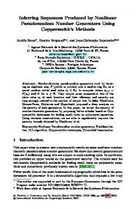
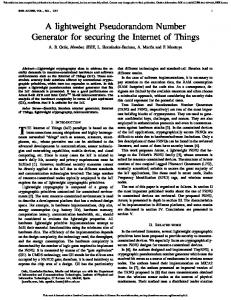
Here, N represents the total number of coordinates tested. As N increases, it is probable that the accuracy of the estimate of the integral increases. The third simulator tested is an efficient exact stochastic simulator of chemical systems with many species and many channels used for biological modeling. This simulator uses the Next Reaction Method algorithm, based on Gibson and Bruck’s improvements to Gillespie’s stochastic simulation algorithm [4,5]. The user specifies a list of chemical species, the species’ initial populations, a list of chemical reactions, and a list of stochastic rate constants associated with the chemical reactions. In each iteration of the simulator’s loop, exponentially distributed random numbers are used to estimate which chemical reaction will next occur and how much time will pass between reaction executions. Many iterations are performed to determine the final state of the chemical system after a specified period of time. Execution time and speedup estimates for each of these simulators is provided in Table I. V. IMPLEMENTATION The design was synthesized for several different values of M, K, and W using the Mentor Graphics placement and routing tool set. The design was targeted for a Xilinx XCV300 FPGA, which has an estimated capacity of 300,000 gates. The Hardware Method can be decomposed into three main sections, the LFSR, the lookup table, and the linear interpolation unit. The size of the LFSR is directly proportional to the parameter M, which defines the size and period of the pseudo-random number sequence generated. A plot of device utilization for the LFSR versus the M factor is given in Fig. 1. The size of the linear interpolation unit is directly proportional to width of each entry in the lookup table, W. A plot of device utilization for the linear interpolation unit versus the W parameter is given in Fig. 2. 40 Function Generators
35
Number of Units Used
TABLE I SIMULATOR SPEEDUP ESTIMATES
Combinational Logic Block Slices DFF's or Latches
30 25 20 15 10 5 0 0
(11)
10
20
Bit Width (W) Fig. 1. A plot of the LFSR device utilization for various values of lookup table bit widths (W).
30
350
TABLE III MEAN SQUARED LINEAR INTERPOLATION ERROR STATISTICS FOR M=1024
Function Generators
Number of Units Used
300
Combinational Logic Block Slices DFF's or Latches
250 200 150 100 50 0 0
10
20 Bit Width (W)
30
Fig. 2. A plot of the linear interpolation unit device utilization for various values of lookup table bit widths (W).
The lookup table would be best implemented on a memory chip, so that lookup table values could be quickly loaded and read. The size of the lookup table is the product of the number of entries in the lookup table, 2K+1, and the size of each entry in the lookup table, W. The final design was targeted for the Wildcard reconfigurable computing PCMCIA card with M=232, K=16, and W=32 [6]. This design consumed 262kB of the Wildcard onboard SRAM for the lookup table and utilized approximately 10% of the total area of the onboard Xilinx XCV300 device.
K 1 2 3 4 5 6 7 8 9 10
Uniform 0 0 0 0 0 0 0 0 0 0
Exponential 12.3934 5.2448 2.1855 0.8933 0.356 0.1368 0.0495 0.0159 0.0037 0
Gaussian 0.5112 0.2029 0.0796 0.0307 0.0116 0.0043 0.0015 4.58E-04 1.03E-04 0
Interpolation error is introduced when the linear interpolation unit estimates a straight line between two points in the cumulative distribution function when a curve actually exists. Table III shows the mean squared linear interpolation error per point for the uniform, exponential and Gaussian distribution functions for various values of K and a fixed M value of 1024. This error primarily depends on the linearity of the cumulative distribution function and the number of entries in the lookup table. Uniform probability distributions have no linear interpolation error because their cumulative distribution functions are linear. Distribution functions wi th non-linearities suffer the largest interpolation error.
VI. RANDOM NUMBER ACCURACY VI. FUTURE WORK The Hardware Method introduces two types of error into the pseudo-random numbers generated, precision error and interpolation error. Precision error is a directly related to W, the number of bits used to represent the random number, and is caused by round off. This error is also present in the floating-point and double-precision floating-point representation of numbers. Increasing W will decrease the precision error. If W is large enough, the numbers generated by the Hardware Method can be more precise than numbers generated by Software Method. The mean-squared precision error per point for various values of W is given in Table II. The data is based on 1000 data points taken from the exponential distribution. TABLE II PRECISION ERROR STATISTICS FOR VALUES OF W
W 4 8 16 24 32
Decimal Precision 1.00000000 0.10000000 0.00100000 0.00001000 0.00000001
Exponential Mean Sq. Err. 0.08085 0.000827 8.31E-05 8.39E-12 8.41E-18
To test the effectiveness of the design, a high speed reconfigurable computing system should be used to measure the simulator speedup when using the Hardware Method. This testing could verify the speedup estimates reported in Table I. Future research could investigate implementing a hardware design that generates numbers in parallel and shares a lookup table. Methods could be developed for better handling discontinuities or discrete probability distribution functions to reduce interpolation error. Implementing a second or third order interpolation method could also be an effective way to reduce interpolation error for particular probability distributions. VII. CONCLUSION An efficient design for generating random numbers from any probability distribution function in an FPGA is given. Generating random numbers in hardware could be an effective way to enhance the performance of simulation applications that require a large amount of random numbers.
As FPGA cost decreases and the capacity of these devices increase according to Moore’s Law, the potential for extremely long sequences of highly accurate pseudo-random numbers generated in parallel will become more feasable. VIII. ACKNOWLEDGEMENTS This work was partially supported by the National Science Foundation via grants #0075792 and #0130843, the University of Tennessee Center for Environmental Biotechnology, and the University of Tennessee Center for Information Technology Research. We gratefully acknowledge their support. XI. REFERENCES [1] R. Jain, The Art of Computer Systems Performance Analysis: Techniques for Experimental Design, Measurement, Simulation, and Modeling, John Wiley & Sons, Inc., NY: 1991, pp. 439-444, 488-489. [2] M. J. S. Smith, Application-Specific Integrated Circuits, Addison-Wesley, MA: 2001, pp. 766-777. [3] K. H. Tsoi, Pilchard User Reference (V0.1), Department of Computer Science and Engineering, The Chinese University of Hong Kong, Shatin, NT Hong Kong: January 2002. [4] D.T. Gillespie, “Exact Stochastic Simulations of Coupled Chemical Reactions,” J. Phys. Chem., vol. 81, 1977, pp. 2340-2361. [5] M. A. Gibson and J. Bruck, “Efficient Exact Stochastic Simulation of Chemical Systems with Many Species and Many Channels,” J. Phys. Chem. A, vol. 409, 2000, pp. 1876-1889. [6] Annapolis Micro Systems, Inc., Wildcard Reference Manual, 1999.