The massively parallel simulation handles collision detection and reaction of particles with ..... i the velocity after the collision can be computed applying friction ν ...
Graphics Hardware (2004) T. Akenine-Möller, M. McCool (Editors)
Hardware-based Simulation and Collision Detection for Large Particle Systems A. Kolb∗ and L. Latta† and C. Rezk-Salama∗ ∗ Computer
Graphics and Multimedia Systems Group, University of Siegen, Germany † 2L Digital, Mannheim, Germany
Abstract Particle systems have long been recognized as an essential building block for detail-rich and lively visual environments. Current implementations can handle up to 10,000 particles in real-time simulations and are mostly limited by the transfer of particle data from the main processor to the graphics hardware (GPU) for rendering. This paper introduces a full GPU implementation using fragment shaders of both the simulation and rendering of a dynamically-growing particle system. Such an implementation can render up to 1 million particles in real-time on recent hardware. The massively parallel simulation handles collision detection and reaction of particles with objects for arbitrary shape. The collision detection is based on depth maps that represent the outer shape of an object. The depth maps store distance values and normal vectors for collision reaction. Using a special texturebased indexing technique to represent normal vectors, standard 8-bit textures can be used to describe the complete depth map data. Alternately, several depth maps can be stored in one floating point texture. In addition, a GPU-based parallel sorting algorithm is introduced that can be used to perform a depth sorting of the particles for correct alpha blending. Categories and Subject Descriptors (according to ACM CCS): I.3.1 [Computer Graphics]: Graphics processors I.3.5 [Computer Graphics]: Boundary representations I.3.7 [Computer Graphics]: Animation
1. Introduction Physically correct particle systems (PS) are designed to add essential properties to the virtual world. Over the last decades they have been established as a valuable technique for a variety of applications, e.g. deformable objects like cloth [VSC01] and volumetric effects [Har03]. Dynamic PS have been introduced by [Ree83] in the context of the motion picture Star Trek II. Reeves describes basic motion operations and basic data representing a particle - both have not been altered much since. An implementation on parallel processors of a super computer has been done by [Sim90]. [Sim90] and [McA00] describe many of the velocity and position operations of the motion simulation also used in our PS. Real-time PS are often limited by the fill rate or the CPU to graphics hardware (GPU) communication. The fill rate is often a limiting factor when there is a high overdraw due to relatively large particle geometries. Using a large number c The Eurographics Association 2004.
of smaller particles decreases the overdraw and the fill rate limitation looses importance. The bandwidth limitation now dominates the system. Sharing the graphics bus with many other rendering tasks allows CPU-based PS to achieve only up to 10,000 particles per frame in typical real-time applications. A much larger number of particles can be used by minimizing the amount of communication of particle data by integrating simulation and rendering on the GPU. Stateless PS, i.e. all particle data can be computed by closed form functions based on a set of start values and the current time, have been implemented using vertex shaders (cf. [NVI03]). However, state-preserving PS can utilize numerical, iterative integration methods to compute the particle data from previous values and a dynamically changing environment. They can be used in a much wider range of applications. While collision reaction for particles is a fairly simple application of Newtonian physics, collision detection can be a rather complex task w.r.t. the geometric representation of
A. Kolb, L. Latta and C.Rezk-Salama / Hardware-based Simulation and Collision Detection for Large Particle Systems
the collider object. [LG98] gives a good overview on collision detection techniques for models represented as CSG, polygonal, parametric or implicit surfaces. There are three basic image-based hardware accelerated approaches to collision detection based on depth buffers, stencil buffers or occlusion culling. However, all these techniques use the GPU to generate spatial information which has to be read back from the GPU to the CPU for further collision processing. The technique presented in this paper uses the “stream processing” paradigm, e.g. [PBMH02], to implement PS simulation, collision detection and rendering completely on the fragment processor. Thus a large number of particles can be simulated using the state-preserving approach. The collision detection is based on an implicit, image based object boundary representation using a sequence of depth maps similar to [KJ01]. Several approaches are presented to store one, two or six depth maps in a single texture. Storing the normal vectors for collision reaction is realized using a texture-based normal indexing technique. The remainder of this paper is organized as follows. Section 2 gives an overview over works related to this paper. The GPU based simulation for large particle systems is described in section 3. Collision detection on the GPU is discussed in section 4. Results and conclusions are given in sections 5 and 6 respectively.
2. Prior work This section describes prior works related to particle systems (PS) and their implementation using graphics hardware (section 2.1). Additionally, we briefly discuss collision detection approaches (section 2.2), techniques to generate implicit representations for polygonal objects (section 2.3) and the compression of normal vectors (section 2.4).
2.1. Stateless particle systems Some PS have been implemented with vertex shaders on programmable GPUs [NVI03]. However, these PS are stateless, e.g. they do not store the current positions of the particles. To determine a particle’s position a closed form function for computing the current position only from initial values and the current time is needed. As a consequence such PS can hardly react to a dynamically changing environment. Particle attributes besides velocity and position, e.g. the particle’s orientation, size and texture coordinates, have generally much simpler computation rules, e.g. they might be calculated from a start value and a constant factor of change over time. So far there have been no state-preserving particle systems fully implemented on the GPU.
2.2. Collision detection techniques The field of collision detection is one of the most active in recent years. Lin and Gottschalk [LG98] give a good overview on various collision detection techniques and a wide range of applications, e.g. game development, virtual environments, robotics and engineering simulation. There are three basic hardware accelerated approaches based on depth buffers, stencil buffers and occlusion culling. All approaches are image based and thus their accuracy is limited due to the discrete geometry representation. Stencil buffer and depth buffer based approaches like [BW03, HZLM02, KOLM02] use the graphics hardware to generate proximity, collision or penetration information. This data has to be read back to the CPU to perform collision detection and reaction. Usually, these techniques use the graphics hardware to detect pairs of objects which are potentially colliding. This process may be organized hierarchically to get either more detailed information or to reduce the potentially colliding objects on a coarser scale. Govindaraju et.al. [GRLM03] utilize hardware accelerated occlusion queries. This minimizes the bandwidth needed for the read-back from the GPU. Again, the collision reaction is computed on the CPU. 2.3. Implicit representation of polygonal objects Implicit representations of polygonal objects have advantages in the context of collision detection, since the distance of any 3D-point is directly given by the value of the implicit model representation, the so-called distance-map. Nooruddin and Turk [NT99, NT03] introduced a technique to convert a polygonal model in an implicit one using a scanline conversion algorithm. They use the implicit representation to modify the object with 3D morphological operators. Kolb and John [KJ01] build upon Nooruddin and Turk’s algorithm using graphics hardware. They remove mesh artifacts like holes and gaps or visually unimportant portions of objects like nested or overlapping parts. This technique generates an approximate distance map of a polygonal model, which is exact on the objects surface w.r.t. to the visibility of object points and the resolution of the depth buffer. 2.4. Compression of normal vectors For collision reaction, an efficient way to store an object’s normal, i.e. the collision normal, at a particular point on the object’s surface is needed. Deering [Dee95] notes, that angular differences below 0.01 radians, yielding some 100k normal vectors, are not visually recognizable in rendering. Deering introduces a normal encoding technique which requires several trigonometric function calls per normal. In our context we need a normal representation technique c The Eurographics Association 2004.
A. Kolb, L. Latta and C.Rezk-Salama / Hardware-based Simulation and Collision Detection for Large Particle Systems
which is space and time efficient. Possible decoding of the vector components must be as cheap as possible, while the encoded data must be efficiently stored in textures. Normal maps store normal vectors explicitly and are not space efficient. Applying an optional DXT-compression results in severe quantization artifacts (cf. [ATI03]). Sphere maps, cube maps and parabolic maps, commonly used to represent environmental information, may be used to store normal vectors. Sphere maps heavily depend on a specific viewing direction. Cube maps build upon a 3D-index, i.e. a point position in 3-space. Parabolic maps need two textures to represent a whole sphere. Additionally, they only utilize the inscribed circle of the texture. 2.5. Other related works Green [Gre03] describes a cloth simulation using simple grid-aligned particle physics, but does not discuss generic particle systems’ problems, like allocation, rendering and sorting of PS. The photon mapping algorithm described by Purcell et.al. [PDC∗ 03] uses a sorting algorithm similar to the odd-even merge sort presented in section 3.3.3. However, their algorithm does not show the necessary properties to exploit the high frame-to-frame coherence of the particle system simulation. 3. Particle simulation on Graphics Hardware
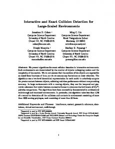
Optionally, in step 4. the particle positions can be sorted depending on the viewer distance to avoid rendering artifacts. The sorting performs several additional rendering passes on textures that contain the particle-viewer distance and a reference to the particle itself. Then the particle positions are transferred from the position texture to a vertex buffer and the particles are rendered as point sprites, triangles or quads. 3.2. Particle data storage The positions and velocities of all active particles are stored in floating point textures using the three color components as x, y and z coordinates. The texture itself is also a render target, so it can be updated with the computed positions and velocities. Since a texture cannot be used as input and output at the same time, we use a pair of these textures and a double buffering technique (cf. figure 1). Depending on the integration algorithm the explicit storage of the velocity texture can be omitted (cf. section 3.3.2). Other particle attributes like mass, orientation, size, color, and opacity are typically static or can be computed using a simple stateless approach (cf. section 2.1). To minimize the upload of static attribute parameters we introduce particle types. Thus the simulation of these attributes uses one further texture to store the time of birth and a reference to the particle type for each particle (cf. figure 1). To model more complex attribute behavior, simple key-frame interpolation over the age of the particle can be applied.
The following sections describe the algorithm of a statepreserving particle system on a GPU in detail. After a brief overview (section 3.1), the storage (section 3.2) and then the processing of particles is described (section 3.3). 3.1. Algorithm Overview The particle simulation consists of six basic steps: 1. 2. 3. 4. 5. 6.
Process birth and death Update velocities Update positions Sort for alpha blending (optional) Transfer texture data to vertex data Render particles
The state-preserving particle system stores the velocities and positions (step 2. and 3.) of all particles in textures, which are also render targets. In one rendering pass the texture with particle velocities is updated, performing a single time step of an iterative integration. Here acceleration forces and collision reactions are applied. A second rendering pass updates the position textures in a similar way, using the velocity texture. Depending on the integration method it is possible to skip the velocity update pass, and directly integrate the position from accelerations (cf. section 3.3.2). c The Eurographics Association 2004.
Figure 1: Data storage using double buffered textures
3.3. Simulation and rendering algorithm 3.3.1. Process birth and death Assuming a varying number of short-living particles, the particle system must be able to process the birth of a new particle (allocation) and the death of a particle (deallocation). Since allocation problems are serial by nature, this cannot be done efficiently with a data-parallel algorithm on the GPU. Therefore an available particle index is determined on the CPU using either a stack filled with all available indices or a heap data structure that is optimized to always return
A. Kolb, L. Latta and C.Rezk-Salama / Hardware-based Simulation and Collision Detection for Large Particle Systems
the smallest available index. The heap data structure guarantees that particles in use remain packed in the first portion of the textures. The following simulation and rendering steps only need to update that portion of data, then. The initial particle data is determined on the CPU and can use complex algorithms, e.g. probability distributions (cf. McAllister [McA00]). A particle’s death is processed independently on the CPU and GPU. The CPU registers the death of a particle and adds the freed index to the allocator. The GPU does an extra pass to determine the death of a particle by the time of birth and the computed age. The dead particle’s position is simply moved to invisible areas. As particles at the end of their lifetime usually fade out or fall out of visible areas anyway, the extra clean-up pass rarely needs to be done. 3.3.2. Update velocities and position Updating a particle’s velocity and position is based on the Newtonian laws of motion. The actual simulation is implemented in a fragment shader. The shader is executed for each pixel of the render target by rendering a screen-sized quad. The double buffer textures are alternately used as render target and as input data stream, containing the velocities and positions from the previous time step.
~vi into a normal component ~v⊥ i and a tangential component k
~vi the velocity after the collision can be computed applying friction ν and resilience ε: k
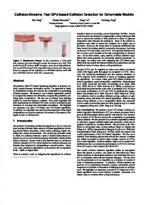
~vi = (1 − ν)~vi − ε~v⊥ i To avoid velocities from slowing down close to zero, the friction slow-down should not be applied if the overall velocity is smaller than a given threshold. Having collider with sharp edges, e.g. a height field, or two colliders close to each other, the collision reaction might push particles into a collider. In this case a caught particle ought to be pushed out in the next simulation step. To handle this situation, the collision detection is done twice, once with the previous and once with the expected position P∗i based on velocity~v∗i . This allows differentiating between particles that are about to collide and those having already penetrated (cf. figure 2). The latter must be pushed in direction of the shortest way out of the collider. This direction can be guessed from the normal component of the velocity: ( � ~v∗i if ~v∗i · nˆ ≥ 0 (heading outside) � ~vi = ∗ if ~v∗ · n ~v⊥ i −~vi i ˆ < 0 (heading inside)
There are several operations that can be used to manipulate the velocity (cf. [Sim90] and [McA00] for more details): global forces (e.g. gravity, wind), local forces (attraction, repulsion), velocity dampening, and collision responses. For our GPU-based particle system these operations need to be parameterized via fragment shader constants. A complex local force can be applied by mapping the particle position into a 2D or 3D texture containing flow velocity vectors~vflow . Stoke’s law is used to derive a dragging force:
P∗i Pi
Pi−1 Pi Pi−2
Pi−1 P∗i
P∗i−1
Figure 2: Particle collision: a) Reaction before penetration; b) Double collision with caught particle and push-back.
~Fflow = 6 π η r(~vi−1 −~vflow ) where η is the flow viscosity, r the particle radius and ~vi−1 the particle’s previous velocity. The new velocity ~vi and position P is derived from the accumulated global and local forces ~F using simple Euler integration. Alternatively, Verlet integration (cf. [Ver67]) can be used to avoid the explicit storage of the velocity by utilizing the position information Pi−2 . The great advantage is that this technique reduces memory consumption and removes the velocity update rendering pass. Verlet integration uses a position update rule based only on the acceleration: Pi = 2Pi−1 − Pi−2 +~a∆2i Using Euler integration, collision reaction is based on a change of the particle’s velocity. Splitting the velocity vector
Verlet integration cannot directly handle collision reactions in the way discussed above. Here position manipulations are required to implicitly change the velocity in the following frames. 3.3.3. Sorting If particles are blended using a non-commutative blending mode, a depth-based sorting should be applied to avoid artifacts. A particle system on the GPU can be sorted quite efficiently with the parallel sorting algorithm "odd-even merge sort" (cf. Batcher [Bat68]). Its runtime complexity is independent of the data’s sortedness. Thus, a check whether all data is already in sequence does not need to be performed on the GPU, which would be rather inefficient. Additionally, with each iteration the sortedness never decreases. Thus, using the high frame-to-frame coherence of the particle order, c The Eurographics Association 2004.
A. Kolb, L. Latta and C.Rezk-Salama / Hardware-based Simulation and Collision Detection for Large Particle Systems
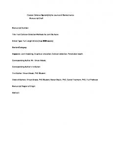
the whole sorting sequence can be distributed over 20 - 50 frames. This, of course, leads to an approximate depth sortedness, which, in our examples, does not yield any visual artifacts. The basic principle of odd-even merge sort is to divide the data into two halves, to sort these and then to merge the two halves. The algorithm is commonly written recursively, but a closer look at the resulting sorting network reveals its parallel nature. Figure 3 shows the sorting network for eight values. Several consecutive comparisons are independent of each other and can be grouped for parallel execution (vertical lines in figure 3).
2D-rotation, texture coordinates are transformed in the fragment shader. 4. Collision detection In this section we describe the implicit object representation used for collision detection (section 4.1). Furthermore, the normal indexing technique (section 4.2) and various approaches to represent depth maps in textures are introduced (section 4.3). 4.1. Implicit model representation We use an image-based technique similar to [KJ01] to represent an objects outer boundary by a set of depth maps. These depth maps contain the distance to the object’s boundary and the surface normal at the relevant object point. Each depth map DMi , i = 1, . . . , k stores the following information:
Figure 3: Odd-Even sorting network for eight values; arrows mark comparison pairs.
The sorting requires 21 log22 n + 21 log2 n passes, where n is the number of elements to sort. For a 1024 × 1024 texture this leads to 210 rendering passes. Running all 210 passes each frame is far too expensive, but spreading the whole sorting sequence over 50 frames, i.e. 1 - 2 seconds, reduces the workload to 4 − 5 passes each frame. The sorting algorithm requires an additional texture containing the particle-viewer distance. The distance in this texture is updated after the position simulation. After sorting the rendering step looks up the particle attributes via the index in this texture. 3.3.4. Render particles The copying of position data from a texture to vertex data is an upcoming hardware feature in PC GPUs. DirectX and OpenGL offer the vertex textures technique (vertex shader 3.0 rsp. ARB_vertex_shader extension). Unfortunately there is no hardware supporting this feature at the moment. Alternatively "über-buffers" (also called super buffers; cf. [Per03]) can be used. This functionality is already available in current GPUs, but up to now it is only supported by the OpenGL API. The current implementation uses the vendor specific NV_pixel_data_range extension (cf. [NVI04]). The transferred vertex positions are used to render primitives to the frame buffer. In order to reduce the workload of the vertex unit, particles are currently rendered as point sprites instead of as triangles or quads. The disadvantage though is that particles are always axis-aligned. To allow a c The Eurographics Association 2004.
1. distance dist(x, y) to the collider object in projection direction for each pixel (x, y) ˆ y) at the relevant object surface point 2. normal vector n(x, 3. transformation matrix TOC→DC mapping from collider object coordinates to depth map coordinates, i.e. the coordinate system in which the projection was performed 4. zscale scaling value in z-direction to compensate for possible scaling performed by TOC→DC The object’s interior is assigned with negative distance values. Assuming we look from outside onto the object and orthographic projection is used, the distance value f (P) for a point P is computed using the transformation TOC→DC : � f (P) = zscale · dist(p0x , p0y ) − p0z , (1) where P0 = (p0x , p0y , p0z )T = TOC→DC P
TOC→DC usually also contains the transformation to texture coordinates. Thus fetching the depth value dist(p0x , p0y ) is a simple texture lookup at coordinates (p0x , p0y ). Taking several depth maps into account, the most appropriate depth for point P has to be determined. The following definition guarantees that P is outside of the collider if at least one depth map has recognized P to be exterior: ( max{ fi (P)} if fi (P) < 0 ∀i f (P) = min{ fi (P) : fi (P) > 0} else where fi (P) denotes the signed distance value w.r.t. depth map DMi . Handling several depth maps DMi , i = 1, . . . , k, f (P) can be computed iteratively: � ( f (P) < 0 ∧ fi (P) > f (P)) ∨ ⇒ ( f (P) ← fi (P)) (2) ( fi (P) > 0 ∧ fi (P) < f (P)) where f (P) is initially set to a large negative value, i.e. P is placed “far inside” the collider.
A. Kolb, L. Latta and C.Rezk-Salama / Hardware-based Simulation and Collision Detection for Large Particle Systems
If P0 = TOC→DC P lies outside the view volume for the current depth map or the texture lookup dist(p0x , p0y ) results in the initial background value, e.g. no distance to the object can be computed, this value may be ignored as invalid vote. Alternatively, if the view volume encloses the complete collider object, the invalid votes can be declared as “far outside”. To avoid erroneous data due to clamping of (p0x , p0y ), we simply keep a one pixel border in the depth map unchanged with background values to indicate an invalid vote. A fragment shader computes the distance using rule (2) and applies a collision reaction when the final f (P) distance is negative. Note, that this approach may have problems with small object details in case of an insufficient buffer resolution. Problems can also be caused by local surface concavities. In many cases, these local concavities can be reconstructed with properly placed depth map view volumes (cf. section 5). 4.2. Quantization and indexing of normal vectors Explicitly storing normal vectors using 8, 16 or 32 bit per component is sufficient within certain error bound (cf. [ATI03]). Since we store unit vectors, most of the used 3space remains unused, though. The depth map representation requires a technique which allows the retrieval of normal vectors using a space- and time efficient indexing method. Indices must be encoded in depth maps and the reconstruction of the normal vector in the fragment shader must be efficient. The normal representation, which is implemented by indexing into a normal index texture, should have the following properties: 1. the complete coordinate space [0, 1]2 of a single texture is used 2. decoding and ideally encoding is time efficient 3. sampling of the directional space is as regular as possible t x0 z0 y0
y
x>0 y>0 z0 y