804
J. Opt. Soc. Am. A / Vol. 26, No. 4 / April 2009
Li et al.
Hardware implementation and calibration of background noise for an integration-based fluorescence lifetime sensing algorithm Day-Uei Li,1,* Richard Walker,1 Justin Richardson,1,2 Bruce Rae,1 Alex Buts,1 David Renshaw,1 and Robert Henderson1 1
Institute for Integrated Micro and Nano Systems, Joint Research Institute for Signal & Image Processing/Integrated Systems/Energy/Civil and Environmental Engineering, School of Engineering, The University of Edinburgh, Edinburgh EH9 3JL, Scotland, UK 2 Imaging Division, STMicroelectronics, 33 Pinkhill, Edinburgh EH12 7BF, Scotland, UK *Corresponding author:
[email protected] Received December 10, 2008; revised January 28, 2009; accepted February 2, 2009; posted February 3, 2009 (Doc. ID 105082); published March 17, 2009 A new integration based fluorescence lifetime imaging microscopy (FLIM) called IEM has been proposed to implement lifetime extraction [J. Opt. Soc. Am. A 25, 1190 (2008)]. A real-time hardware implementation of the IEM FLIM algorithm suitable for single photon avalanche diode arrays in nanometer-scale CMOS technology is now proposed. The problems of reduced pixel readout bandwidth and background noise are studied and a calibration method suitable for FPGA implementation is introduced. In particular, the relationship between signal-to-noise ratio and background noise is considered based on statistics theory and compared with a rapid lifetime determination method and maximum-likelihood estimator with–without background correction. The results are also compared with Monte Carlo simulations giving good agreement. The performance of the proposed methods has been tested on monoexponential decay experimental data. The high flexibility, wide range, and hardware friendliness make IEM the best candidate for system-on-chip integration to our knowledge. © 2009 Optical Society of America OCIS codes: 030.5260, 030.5290, 040.6070, 170.2520, 170.3650, 170.6920.
1. INTRODUCTION Fluorescence lifetime imaging (FLIM) is widely used in biology, chemistry, medicine, medical research, and medical diagnosis [1–5]. As shown in Fig. 1(a), a laboratory two-photon microscopy (TPM) FLIM experiment usually contains a titanium-sapphire femtosecond laser system as an excitation source, a photomultiplier tube (PMT) as a fluorescence emission detector, a card for photon counting and as a control system, a PC as a user interface, and fluorescence lifetime analysis software. These existing systems are mainly aimed at research applications and provide excellent time resolution down to tens of picoseconds and excellent light sensitivity [1], although they are quite expensive and cumbersome. Another serious challenge is that the available computational methods for generation of lifetime map images such as the iterative least-square method (LSM) or maximum-likelihood estimation (MLE) [6,7] are very time-consuming, making real-time imaging impossible. A new FLIM algorithm considering the instrument response based on the Laguerre expansion technique [8] speeds up lifetime calculations but the computation time increases with imager size. However, in many applications such as microfluidic mixing [3,4], exploratory biological experiments, and clinical diagnosis with endoscopy, it is desirable to monitor the instantaneous biochemical reactions to provide quick feedback to corresponding manipulations. The slow speed of 1084-7529/09/040804-11/$15.00
LSM-based software analysis tools becomes the bottleneck and has driven the recent development of noniterative, compact, and fast real-time time-domain FLIM systems [9–18] and real-time frequency-domain FLIM algorithms and systems [19–22]. An interesting analog circuit was proposed [17] to calculate lifetimes for singlemolecule microscopy, however, it did not reveal how to remove background noise. In such applications with low fluorescence emission, background-to-signal ratio will be relatively significant. Commercial applications increasingly demand compact, low-cost, and even portable system-on-chip (SOC) FLIM solutions. Fortunately, high accuracy time resolution can be achieved by exploiting single photon avalanche diode (SPAD) detectors. The feasibility, features, and excellent performance of SPADs in standard complementary metal-oxide-semiconductor (CMOS) technology accompanied by integrated digital readout circuitry [23–28] promise on-chip lifetime extraction and processing. As excitation sources, AlInGaN UV micropixelated light-emitting diodes (micro-LEDs) can be bump-bonded to the digital counters and LED drivers [12] in the general direction of lab-on-chip. In the past, rapid lifetime determination (RLD) methods were thought to be the simplest algorithms [10], and suitable for real-time applications. A video-rate FLIM was proposed using optomechanical delay control for RLD [14], however, its © 2009 Optical Society of America
Li et al.
Fig. 1. (Color online) (a) Laboratory FLIM. (b) FLIM system-on-chip.
cumbersome optical setup makes it difficult to image a wide range of fluorophore lifetimes and an electronically controllable delay would be preferable [15]. For this purpose, we evaluated the possibility of applying RLD either on-chip or on-FPGA and concluded that RLD can be implemented on FPGA with lookup tables (LUTs) of natural logarithmic or other functions if overlap gating is used [11,13]. However, to build a LUT on-FPGA covering a wide range of lifetimes is inefficient and it is necessary to develop more hardware- or FPGA-friendly algorithms. Moreover, in realistic applications, although video-rate lifetime imagers can provide quick feedback, the raw data must still be processed with software for detailed scientific research. Also, large fluorescence lifetime differences exist in Föster resonance energy transfer (FRET) experiments, and there is an increasing demand for detectors to measure coexisting samples with large lifetime differences. The lifetime range of the imager is therefore from hundreds of picoseconds to tens of nanoseconds. To accommodate these needs, the measurement window is set at several times of the largest lifetime of the samples [with a laser pulse repetition (LPR) rate of several megahertz or a measurement window of hundreds of nanoseconds] [1]. It is a challenging task for the standard RLD to meet such requirements, especially when the lifetime is much less than the measurement window. Therefore, to achieve hardware friendliness and wide range of resolvability, a new integration based algorithm called integration for extraction method (IEM) has been proposed [9] and its performance was successfully verified on single-exponential and multiexponential experimental data obtained by conventional laboratory FLIM instruments. The IEM-based system allows minimum software calculation requirements on both a scanning and a wide-field system. The best way is to make the system selectable and controllable by the end users. The main role of real-time IEM algorithms is for exploratory biological experiments by adapting a wide-field microscope to accommodate the SPAD array. More precise measurements on a scanning system using IEM or software can follow if necessary. As mentioned earlier, the fully integrated FLIM system is comparable to a TPM–TCSPC (time-correlated singlephoton counting) system since raw data for precise analysis is also available and light sources and detectors with comparable FWHM are employed. Figure 1(b) shows the
Vol. 26, No. 4 / April 2009 / J. Opt. Soc. Am. A
805
SOC solution suited to lab-on-chip applications, which is intended to replace the system of Fig. 1(a). The first objective of this paper is to introduce an efficient hardware implementation of IEM [9]. By minimizing the digital circuitry we aim to provide in-pixel or on-FPGA (field programmable gate array) lifetime computation compatible with the increasing numbers of pixels in SPAD arrays (beyond 10,000 in the future). The second objective is to address the problems of inaccurate lifetime extraction caused by the background noise of the SPADs. The dark count rate (DCR) of the PMT used in the measurement setup of [9] is about 2 kHz at a temperature of 25° C, which does not have a serious impact on the accuracy of lifetime calculation algorithms since the photon count rate (PCR) at such a single sensor system is much higher than the DCR. Moreover, without using background correction, IEM still provides accurate lifetime calculations. Its insensitivity to the background noise will be explained in Subsection 2.A. Recently proposed CMOS SPAD structures have reduced the DCR down to hundreds of hertz to several kilohertz at room temperature [24–28] comparable to some state-of-the-art PMTs. However, to achieve parallelism for wide-field microscopy, large arrays of miniaturized SPADs are necessary. It might be argued that increasing light intensity or increasing the LPR rate could improve the ratio of the total photon count caused by fluorescence emission (effective signal count Nc) over that caused by dark count noise (background noise count Nb). This technique is applicable to single-SPAD detection systems with the dead time of a SPAD of tens of nanoseconds, where a DCR of hundreds of kilohertz is perhaps still acceptable. However, as Fig. 2 shows, for modern applications requiring large SPAD arrays, the system becomes readout-bandwidth or framerate limited. Moreover, in FLIM applications, it is necessary to avoid the pileup effect [1], which usually keeps the PCR of SPADs much smaller than the readout bandwidth and this imposes more serious constraints than 3D ranging applications [23]. On the other hand, there are an increasing number of noisy pixels as the SPAD arrays get larger due to silicon defectivity mechanisms, and which cannot simply be solved by applying pixel interpolation– extrapolation method to improve the images due to the requirements of FLIM. In Fig. 2, the frequency margin ⌬f between the DCR of the noisy pixels and the PCR is becoming smaller as SPAD arrays get larger, which makes the ratio of Nc over Nb decrease. Therefore, in order to integrate IEM with such system requirements, the algorithm should include the effect of high background noise. The importance of developing this theory before the system integration is that we can predict and optimize
Fig. 2. (Color online) Relationship between DCR and signal readout bandwidth.
806
J. Opt. Soc. Am. A / Vol. 26, No. 4 / April 2009
the parameters [29–31], such as the number and width of channels, the depth of memory, and hardware usage according to the required accuracy. In this paper, we start by considering single-exponential decay for simplicity. The single-exponential assumption allows a proper comparison of various fitting algorithms. We first derive the error equations for IEM using Romberg’s integration rule to illustrate the impact of background noise. And we also propose a hardware noise calibration technique based on the assumption that background noise is white in the time domain since it is uncorrelated to the excitation light source. The performance of the proposed methods has been tested on monoexponential experimental data obtained by CMOS SPAD pixels. Because the measurements show that the possibility of after pulsing is extremely low for our CMOS SPADs, the after-pulsing effect is not included in the analysis. Although this paper is mainly motivated by the reduced ratio of the PCR over DCR for larger SPAD arrays, the algorithms can be generalized to include uncorrelated noise caused by ambient light sources.
2. THEORY A. Simpler IEM Formulations for Hardware Implementation When the FWHM of the instrumental response function (IRF) over the lifetime is much less than 1, we can assume the fluorescence decay function f共t兲 = A exp共−t / 兲 with being the lifetime. For the usual measurement setup in a laboratory, the FWHM is of the order of hundreds of picoseconds, it is reasonable if we target a lifetime larger than 500 ps. Figure 3(a) shows M time bins (bin width of h) generated by the time-to-digital converters (TDCs) in the photon counting circuitry and also the
Li et al.
fluorescence histogram. With the assumption of singleexponential decay, the lifetime is related to the decay function as
共f0 − fM−1兲 =
冕
M−1
tM−1
f共t兲dt ⬵ h
兺 Cf,
共1兲
j j
j=0
t0
where fj = f共tj兲, j = 0 , . . . , M − 1, and Romberg’s integration coefficient Cj = 关1 / 2 , 1 , . . . , 1 , 1 / 2兴 is used. Multiply Eq. (1) on both sides by the factor 共1 − e−h/兲 to obtain M−1
IEM h
兺
=
=
M−1
兺 N − 共N
C jN j
j=0
N0 − NM−1
j
=
0
+ NM−1兲/2
j=0
N0 − NM−1
Nc − 共N0 + NM−1兲/2 N0 − NM−1
共2兲
,
where Nj is the number of counts in the jth time bin and Nc is the total effective signal count. To implement Eq. (2) with hardware, we only need two counters (one for Nc and the other for N0 + NM−1) and one subtracter for the numerator and one up–down counter for the denominator. The hardware implementation is shown as Fig. 3(b). In Fig. 3(b), a K-bit register is used to latch the results from the subtracter when the up–down counter reaches a value of 共3兲
N0 − NM−1 = 2L ,
where L is an integer. By this arrangement, we do not even need digital division by only taking the first 共K − L兲 most significant bit (MSB) bits of the register or more than 共K − L兲 MSB bits for decimal accuracy. For low counts, the histogram is almost white and N0 ⬃ NM−1, and this condition is easily avoided in hardware implementation. For example, the user can set a photon count rate threshold PCRth and when PCR is less than PCRth, the system will display a black pixel on the screen. Compared with Eq. (6) in [9], which we rewrite as
IEM h
=
冋
共M−1兲/2
共N0 + NM−1兲 + 4
兺
共M−3兲/2
N2i−1 + 2
i=1
3共N0 − NM−1兲
兺 i=1
N2i
册
, 共4兲
Fig. 3. (Color online) (a) Single-exponential decay and concept of IEM and (b) hardware implementation of IEM.
where M is odd, Eq. (2) is much easier to implement inpixel or on-FPGA, because fewer counters are needed and we do not need to use so many logic gates by locating photon counts in the second and third terms of Eq. (4) and doing the division-by-3. Therefore the hardware and chip area can be greatly reduced. The hardware implementation shown in Fig. 3(b) is much simpler than previously proposed video-rate systems [14,15]. Also, since the timing data can be compressed in the counters by Eq. (2), the input/output (IO) data rate is more relaxed. Even if divisions in Eq. (2) are done on software rather than on hardware with Eq. (3), IEM is much easier than available realtime algorithms [18–22].
Li et al.
Vol. 26, No. 4 / April 2009 / J. Opt. Soc. Am. A
B. Impact of Background Noise on IEM In applying large advanced CMOS SPAD arrays, the smaller ratio of the PCR over DCR increases the bias of the lifetime estimators if correction measures are not taken. According to the central limit theory, the spread can be reduced as the number of photons increases, but the bias can never be reduced in the same way. Figure 4 verifies this conclusion and shows how the dark count influences the precision / and accuracy ⌬ / of the MLE [29,30] by the theory with a solid curve and Monte Carlo simulations with open circles and crosses. The total effective signal counts and total background noise counts are Nc = 217 and Nb = 104, respectively. If Nb is zero, ⌬ / = 0 for MLE. As Nb = 104, 7% of total count, ⌬ / degrades significantly to less than 22 dB, and / degrades as well. Now we increase the memory space and store more photon counts Nc = 8 ⫻ 217 and Nb = 8 ⫻ 104; the precision is indeed improved by 9 dB with the accuracy curve still fixed. Using IEM we assume that the timing jitter of the TDCs with phase-locked loops is negligible [9]. With white dark count noise (assumed as an independent Poisson process from the time-correlated signal), the fluorescence decay should be modified as f共t兲 = A exp共−t / 兲 + Nb / 共Mh兲, 0 艋 t 艋 Mh, and A = Nc / 关共1 − e−Mh/兲兴. Now the second term of f共t兲 becomes parasitic such that we cannot separate it from the pure exponential function. The recorded variables Nj are independently Poisson distributed with a re共j+1兲h spective mean value ENj = 兰jh f共t兲dt and standard devia1/2 tion Nj = 共ENj兲 , and we thus have ENj = Ncx 共1 − x兲共1 − x 兲 j
M −1
+ N bM
−1
=
Nj2 ,
共5兲
where x = exp共−h / 兲. From Eq. (2), we have M−1
IEM h
j
=
=
j
j=0
j
j
j=0
EN0 − ENM−1 + N0 − NM−1 ¯ 共1 + u/U ¯兲 U V共1 + v/V兲
⬵
=
¯ + u U V + v
¯ 共1 + u/U ¯ − v/V兲 U V
兺
CjENj =
,
共6兲
where
Nc 共1 + x兲共1 − xM−1兲 2
j=0
1−x
M
Nb共M − 1兲 M
= U + B,
M−1
u =
兺 C N , j
共7b兲
j
j=0
Nc共1 − x兲共1 − xM−1兲
V = EN0 − ENM−1 =
1 − xM
共7c兲
,
v = N0 − NM−1 ,
共7d兲
and U = Nc共1 + x兲共1 − xM−1兲 / 关2共1 − xM兲兴, B = Nb共M − 1兲 / M. Equation (6) can therefore be rewritten as
IEM =
h共1 + x兲 2共1 − x兲
冋
= 1+
冋
冉 冊冉 B
1+
1 12
⬵ 1+
1
U
12
␣2 +
B
U
B U
u
冉
−
¯ U
冊 册冉 冊冉
1+
␣2 + O共␣4兲
冉 冊冉
u
−
¯ U
v V
B
1+
冊冉 冊册 冉 1
1+
v V
U
1+
12
u ¯ U
␣2 + 1 +
= 1+
⌬
−
1 12 +
v V
冊 冊
冊
␣2
,
共8兲
where ␣ = h / and the Taylor’s series expansion is used on h共1 + x兲 / 关2共1 − x兲兴. The accuracy and precision of the IEM are defined as ⌬IEM
IEM
1 =
12 1
=
B
␣2 +
冉冊 h
U
冉
2
12
+
1 1+
12
IEM
IEM
冊
Nc M共1 + x兲共1 − xM−1兲
1
2
h
12
1
12 1
= 1+
冋
␣2
h
B
1+
共9兲
,
冊冉 冊冉 冋 冉 冊册 冉
= 1+
U
u ¯ U
−
v V
冊
2
12
⫻ 1+
respectively, and
␣2
Nb 2共M − 1兲共1 − xM兲
冋 冉 冊册
⫻ 1+
Fig. 4. (Color online) Precision and accuracy curves for the MLE with (Nc = 217, Nb = 0), (Nc = 217, Nb = 104), and (Nc = 8 ⫻ 217, Nb = 8 ⫻ 104), respectively.
+
共7a兲
⫻ 1+
M−1
兺 C EN + 兺 C N
M−1
¯ = U
807
Nb 2共M − 1兲共1 − xM兲 Nc M共1 + x兲共1 − xM−1兲
册
a,
共10兲
808
J. Opt. Soc. Am. A / Vol. 26, No. 4 / April 2009
u
a = M−2
兺
Nj2 =
¯ U
−
v V
Nc共1 − x兲 1−x
j=1
M
Li et al.
冑冉 冊 冉 冊 兺 冉 冊 1
1
=
¯ 2U
−
V
2
N02
共x + x2 + ¯ + xM−2兲 +
The precision of the IEM can easily be obtained by combining Eqs. (5), (7), and (11). It is clear that the accuracy of Eq. (9) is a function of the ratio Nb / Nc, therefore it cannot be improved by simply increasing the laser intensity or measurement time. And the precision of Eq. (10) is no longer simply proportional to the square root of N−1 c . It is a function of Nc and Nb / Nc, and it deteriorates as Nb gets larger. If the ratio Nb / Nc is fixed, then the precision / ⬀ N−1/2 . Figures 5(a) and 5(b) show the accuracy and c precision curves versus measurement window 共Mh兲 in for the 128-bin IEM and two-gate RLD (with a gate width wg = 64h) at (Nc = 217, Nb = 102) and (Nc = 217, Nb = 104), respectively. The theoretical results marked as solid curves are compared with Monte Carlo simulations marked with open circles (IEM) and triangles (RLD-2), giving good agreement and proving the correctness of Eqs. (9) and (10). It is clear that the accuracy curves are more sensitive to the background noise. Here we define a new precision value for SNR plots as Precision ⬅
冑
2
+ ⌬2
2 M−2
1
+
¯ U
M
¯ 2U
j=1
M−2 Nb =
Nc共x − xM−1兲 1−x
1
1
Nj2 +
M
+
+
V
2 2 NM−1 ,
Nb共M − 2兲 M
.
共11兲
best resolvability for a wide range of lifetimes in cases of Nb = 0, its Monte Carlo simulations show more sensitivity than the IEM to the background noise. Precision and accuracy curves of IEM and MLE for Nc = 0.99⫻ 217 and Nb = 0.01⫻ 217 are also shown in Fig. 6(b). For practical cases with nonzero Nb, the integration based IEM shows
共12兲
.
It is convenient to determine the optimal parameters with this definition of precision. The optimal points for the 128bin IEM and two-gate RLD precision curves are located at h = 0.2 and wg = 2.5, respectively, at Nb ⬃ 0. The signalto-noise ratio (SNR) for RLD is better than IEM in the range of Mh / ⬍ 10, while IEM dominates in the range of Mh / ⬎ 10. Considering the limitation of pileup effects to the system, in which we have at most one photon count per pixel for ten frames with frame rate 共FR = 1 MHz兲, or PCR= 100 kHz, and if a conservative DCR= 20 kHz is taken, Nc can be obtained as Nc = 共PCR − DCR兲TM = TMPCR − Nb ⇒
Nb Nc
DCR =
PCR − DCR
= 0.25,
共13兲
where TM is the measurement time, which can be easily obtained by implementing a counter in the photon counting module, TM = NF / FR, and NF is the number of frames this counter accumulates. For larger arrays with much more than 16 pixels per column and the same DCR, Nb / Nc becomes even larger. With Nb / Nc larger than 25%, the accuracy is much smaller than 22 dB. If we take Nb / Nc = 0.25, and the number of bits of the register used to store the total count of 共Nc + Nb兲 is 17 bits, the precision and accuracy curves for the 128-bin IEM and 128-bin MLE with Nc = 0.8⫻ 217 and Nb = 0.2⫻ 217 are shown in Figs. 6(a) and 6(b), respectively. In this case, the accuracy is down to less than 12 dB. Although the MLE has the
Fig. 5. (Color online) Precision and accuracy curves for the 128bin IEM and two-gate RLD with (a) Nc = 217, Nb = 102, and (b) Nc = 217, Nb = 104.
Li et al.
Vol. 26, No. 4 / April 2009 / J. Opt. Soc. Am. A
809
discussion above, the accuracy of algorithms is the dominating factor in cases with low Nc to Nb ratio. And since the accuracy depends on the mean value instead of the fluctuations of photon counts, we can make use of a background count collector to remove the unwanted term Nb共M − 1兲 / M in the numerator of Eq. (7a). This is equivalent to subtracting C0 from the recorded count on each bin. Assume that the temperature of the system is controlled such that the dark count rate is at a fixed level. Similarly to the calibration phase of analog-to-digital converters (ADCs) before normal operation, we can reuse the same hardware of Fig. 3(b) to do background noise counting, and the result Nb0共M − 1兲 / M is stored in the K-bit register, where Nb0 is the total noise count during background noise measurement. As shown in Fig. 7, we use a new counter to calculate the measurement time TM0, and the measured information Nb0 and TM0 are stored in a memory table. In the lifetime calculation phase, when the up–down counter storing N0 − NM−1 reaches a value of 2L, it sends a trigger signal to stop the elapsed time measurement counter storing NF. The output of this counter is then connected to the memory table to output a noise count for calibration. A K-bit subtracter is used to smooth the noise count, and as before the first 共K − L兲 bits are the calculated lifetime. Without knowing the exact DCR, the ¯ of Eq. (7a) can still be calibrated as mean value term U Nb0 = TM0DCR = NF0DCR/FR ⇒ Nb = Nb0TM/TM0 = Nb0NF/NF0 ⬵ Nb0 , ¯ = U cal
Nc 共1 + x兲共1 − xM−1兲 2 −
1−x
M
Nb0NF共M − 1兲 MNF0
+
⬵ U,
Nb共M − 1兲 M 共14兲
where NF0 is the number of frames for the background measurement time and FR is the frame rate introduced
Fig. 6. (Color online) Precision and accuracy curves for the (a) 128-bin IEM and two-gate RLD and (b) 128-bin IEM and 128-bin MLE with different Nb / Nc ratios under Nc + Nb = 217.
its superiority over RLD and MLE in terms of accuracy. The other advantages of IEM are: it does not need iterative root calculations of M-order polynomials as MLEs and its hardware implementation in-pixel or on-FPGA is much easier than RLD. C. Hardware Calibration In most practical lifetime analysis methods background is treated as another fitting parameter or taken into account by subtraction of a DC background value C0 共=Nb / M兲 from the data, and these are easy to do by software. However, for faster real-time imaging, it is desirable that a hardware calibration technique can be integrated into the system. It makes more sense to subtract the background by generating the required C0 through available counts than to treat background as a fitting parameter. From the
Fig. 7. (Color online) Hardware implementation of background noise calibration.
810
J. Opt. Soc. Am. A / Vol. 26, No. 4 / April 2009
Li et al.
earlier. The measured time in normal operation mode TM (or NF) is compared with NF0 on the memory table and the closest one is chosen. With this arrangement, the accuracy is equivalent to cases without Nb. D. Error Analysis of IEM–RLD–MLE with Background Noise Calibration With only white background noise, the recorded variables Dj are still independently Poisson distributed with re共j+1兲h spective mean value EDj = 兰jh Nb0 / 共Mh兲dt and standard deviation Dj = 共EDj兲1/2, and we thus have EDj = Nb0M
−1
=
Dj2
M−1
¯u =
= N bM .
IEM,cal =
=
=
M−1
CjENj +
j=0
冉兺
M−1
兺
C j N j −
j=0
M−1
CjEDj +
j=0
兺 C D j
j=0
j
U共1 + ¯u/U兲
冉
V共1 + v/V兲
¯a =
IEM,cal IEM,cal
冑冉
IEM,cal
1
2U
−
V
冊
2
N02 +
Q共x兲 =
冉 冊 冉 冊兺 D0 2U
2
1
+
共Nj2 + Dj2兲 +
j=1
共1 − xM兲共x + xM兲 共1 − x兲共1 − xM−1兲2共1 + x兲
, 2
Z共x兲 =
In Eq. (21), if Q共x兲 dominates, the precision is proportional to 1 / 冑Nc, whereas if Z共x兲 dominates, the precision is proportional to 冑Nb / Nc = 冑Nb / Nc / 冑Nc = / 冑Nc. We can conclude here that under a certain light intensity ( is a fixed value), the precision can be improved 3 dB by doubling Nc as long as the system has enough memory space to store the doubled total count 共Nc + Nb兲. The same hardware background calibration mechanism can also be applied to RLD if it is implemented onFPGA. Neglecting the details of derivation for simplicity, the precision equation is as
RLD,cal
=
wg冑Nc
冑
2 + y + y−1 +
Nb Nc
U
共17兲
j
12
冉
1
1 2U
+
V
冊
U
−
v
12
12
⌬IEM
IEM ¯u
␣2
U
冉 冊
−
2 =
M共1 − x2兲2共1 − xM−1兲2
共19兲
,
Nb=0
v V
¯a ,
2
2U
冊
2
h
12
DM−1
V
共18兲
Nb 关2共M − 1兲共1 − x兲2 + x2 + 1兴共1 − xM兲2 Nc
¯u
1+
.
=
1
2 NM−1 +
冊
2
h
= 1+
2
V
冉冊 冏 冏 冉 冊冉 冊 冋 冉 冊册 1
=
+
冊
v
−
2
h
= 1+
2 M−2
U
¯u
1
共16兲
1
1+
1
⌬
= 1+
冊
,
冉
冋 冉 冊 册冉
⬵ 1+
EN0 − ENM−1 + N0 − NM−1
RLD,cal
2共1 − x兲
⌬IEM,cal
M−1
兺
h共1 + x兲
Therefore, we have
h
j
j=0
Comparing Eq. (16) with Eq. (6), and also Eq. (17) with Eq. (7b), it is obvious that we are trading some precision for accuracy since Nj and Dj are independently Poisson distributed, and
¯ of Eq. (6) and from By calibrating the mean value term U Eq. (14), we have
IEM,cal
兺 C D .
j=0
共15兲
−1
兺
M−1
C j N j −
冑N c
共20兲
冑Q共x兲 + Z共x兲, 共21兲
.
MLE,cal
MLE,cal
冑 冑
=
2
M 2
共1 − x兲 共1 − x 兲
h Nc
冦
1
Nb 2P共x兲 +
xG共x兲
2
Nc x 关G共x兲兴
2
冧
,
x = exp共− t/兲, G共x兲 = 1 − M2xM−1 + 共2M2 − 2兲xM − M2xM+1 + x2M ,
关共1 + y兲2 + 共1 + y−1兲2兴, 共22兲
where y = exp共−wg / 兲, and wg is the gate width. For MLE, also neglecting the details of derivation, the precision equation with the same background calibration can be obtained as
P共x兲 = 关1 − 共M + 1兲xM + MxM+1兴关− M + 共M + 1兲x − xM+1兴 +
共1 − x兲2共1 − xM兲2 6共M + 1兲−1共2M + 1兲−1
.
共23兲
From Eqs. (20)–(23), it can be derived that the SNR of IEM is less sensitive to the background noise. From Eq. (13), it is possible that Nb / Nc Ⰷ 1 for low fluorescence
Li et al.
Fig. 8. (Color online) Precision and accuracy curves with background correction for the 128-bin IEM, 128-bin MLE, and twogate RLD with Nb / Nc = 7.63 and Nc = 217.
emission cases 共PCR Ⰶ 100,000兲. Figure 8 shows the precision and accuracy curves with background calibration for 128-bin IEM, 128-bin MLE, and two-gate RLD with Nc = 217, Nb = 106. The theoretical results marked as solid curves are compared with Monte Carlo simulations marked with open circles, crosses, and triangles, giving good agreement and proving the correctness of Eqs. (19)–(23). It is clear the accuracy is kept the same with cases without background noise. Unlike the cases with Nb ⬃ 0, the peak SNRs of RLD and MLE (with their optimal SNR ranges shrinking) now less than that of IEM indicates that IEM is less sensitive to background noise. For MLE, increasing M does not improve the range of resolvability significantly as in cases of low background noise. It seems this calibration technique can be utilized without limit for IEM, however, to get the same SNR the memory usage and measurement time increase and require much higher laser intensity making the measurement inefficient. A reasonable DCR should be much lower than the PCR. Without calibration, none of the above algorithms can deal with cases for Nb / Nc Ⰷ 1. For cases with limited hardware resources, we can also use Eqs. (9), (10), (19), and (20) and a simple calibration algorithm introduced in [9] to do the image postprocessing.
Vol. 26, No. 4 / April 2009 / J. Opt. Soc. Am. A
811
cence emission is captured by a SPAD array fabricated in 0.13 m CMOS imaging process mounted on a daughter board. Figure 9(a) and 9(b) shows two measured histograms detected by two pixels. The one in Fig. 9(a) is close to the average noise level, while that in Fig. 9(b) is obtained by a much noisier pixel. The noisy pixel is deliberately chosen to evaluate how much noise IEM can tolerate. The dark count noise of the SPAD mainly contributes to the noise floor. To calculate the lifetime, the histogram should be corrected by subtracting the background noise. On the FPGA, this is easily done by the method introduced above or simply subtracting an average count NF of K bins on the noise floor (the flat part of the histogram in Fig. 9) since the delay from the first bin to the bin containing the peak is kept the same through the whole SPAD array. According to the statistics theory, when the number of bins K used to calculate NF is equal to M, these two methods are equivalent. When K is much smaller than M, the SNR of the calibrated lifetime deteriorates. The worst case is K = 1, only using the count on a single bin as a reference. Taking the noisier pixel as an example, Figs. 10(a)–10(c) show the calibrated lifetimes versus NF for different algorithms with measurement window MW = 17 ns 共⬃1兲, MW = 85 ns 共⬃5兲, and MW = 156 ns 共⬃9兲, respectively. The mean value of NF is 3400 counts, and a range of 20 times the standard deviation is chosen. The measurement windows (from the peak) are chosen to be where the SNR of RLD is higher than that of IEM as shown in Fig. 5(a) to demonstrate that the higher flexibility and wider range of IEM is indeed much better for system integration. In Fig. 10(a) the measurement window for all algorithms is taken at one lifetime. Without background correction, the calculated lifetimes for IEM, MLE, and RLD are IEM,0 = 18.0 ns, MLE,0 = 17.7 ns, and RLD,0 = 17.8 ns, respectively. At this measurement window, the sensitivities of all algorithms are 0.4 ps per count. At MW = 5 (optimal condition for RLD) as in Fig. 10(b), without background calibration, the calculated lifetimes for IEM, MLE, and RLD are IEM,0
3. EXPERIMENTAL RESULTS Measurements of the decay of Catskill Green quantum dots (Q dots) (with an emission wavelength of 548 nm, from Evident Technologies) mounted on a microcavity slide have been made to test the proposed IEM noise calibration algorithm. The CdSe/ ZnS Q dots are held in a solution of toluene with a concentration of 61.3 nmol/ ml. The laser pulse rate (LPR) (PicoQuant pulsed diode laser with wavelength of 470 nm) is 2.5 MHz, and the average output power is 0.12 mW. Florescence decay curves were recorded on a time scale of 400 ns, resolved into 4096 channels. With a LPR of 2.5 MHz, there is no bleedthrough observed on measured histograms. The fluores-
Fig. 9. (Color online) Fluorescence histograms detected by two CMOS SPADs.
812
J. Opt. Soc. Am. A / Vol. 26, No. 4 / April 2009
Li et al.
Fig. 10. (Color online) Calculated lifetimes with background correction versus NF for different algorithms with a mean NF of 3400 and MW= 共a兲 17, (b) 85, and (c) 156 ns. Calculated lifetimes with background correction versus NF for different algorithms with a mean NF of 900 and MW= 共d兲 17, (e) 85, and (f) 156 ns.
= 21.7 ns, MLE,0 = 25.7 ns, and RLD,0 = 27.5 ns, respectively. The sensitivities are 1.4, 2.6, and 3.4 ps per count for IEM, MLE, and RLD, respectively. In an exaggerated range of NF (about 20 times the standard deviation around the mean count), the variation of the calibrated lifetime is 8%, 15%, and 20%, respectively. This means that even for a higher–lower NF, IEM gets more accurate results, and we can therefore use a smaller K or a smaller memory LUT on-FPGA to reduce hardware usage. The calibrated lifetime of IEM is about 17 ns, which is in a good agreement with the data provided by the manufacturer. At MW = 9 as in Fig. 10(c), however, without background correction, the calculated lifetimes are IEM,0 = 25.0 ns, MLE,0 = 39.0 ns, and RLD,0 = 46.9 ns, respec-
tively. The sensitivities are 2.5, 10, and more than 40 ps per count for IEM, MLE, and RLD, respectively. However, in this case, even when a very accurate NF is provided for background correction (around 3400 counts), the calibrated lifetime of RLD is far from the reasonable range. A big error is caused. Figures 10(d)–10(f) show the calibrated lifetimes of the quieter pixel versus NF for different algorithms with measurement window MW = 17 ns 共⬃1兲, MW = 85 ns 共⬃5兲, and MW = 156 ns 共⬃9兲, respectively. The mean value of NF is 900 counts, and a range of 20 times the standard deviation is chosen. The calculated lifetimes without background correction for IEM, MLE, and RLD are also listed. The calculated lifetime using IEM is also around 17 ns, giving good consistency with
Li et al.
that obtained by the noisier pixel. Figures 10(a)–10(f) clearly show that with or without background correction for all algorithms, IEM gets much more accurate results as Eqs. (9) and (21)–(23) predict, in good agreement with Figs. 5, 6, and 8, and its range of resolvability is the most insensitive to background noise. More uniform lifetime images can therefore be generated showing the suitability of IEM for widefield imaging.
4. CONCLUSIONS We have modified our previously proposed FLIM algorithm called IEM as Eqs. (2) and (3) for hardware implementation. With the modifications, the hardware resources can be greatly reduced without sacrificing too much precision. Without iteration, IEM offers direct calculation of lifetime and makes real-time imaging feasible. An interesting result of our study is that optimum performance considering both accuracy and precision at low background noise can be obtained at h = 0.2. When integrated with large CMOS SPAD arrays with an increasing number of noisy pixels, IEM shows its superior accuracy over MLE and RLD. Low PCR to DCR ratio renders MLE and RLD inaccurate except in a very limited range of lifetimes. We derived the error equation for IEM with existing background noise and the theoretical results are compared with Monte Carlo simulations, giving good agreement. We also proposed a hardware background noise calibration to correct the accuracy. Its accuracy and precision equations are also derived and compared with Monte Carlo simulations. The error equations for RLD and MLE with background correction are also derived for comparison. The proposed calibration is verified on measured histograms of Q dots using 0.13 m CMOS SPAD arrays and the calculated lifetime is in a good agreement with the data provided by the manufacturer. With background correction for all three algorithms, IEM still shows its superior performance over MLE and RLD. The higher flexibility, wider range of resolvability, and hardware friendliness make IEM the best candidate for realtime FLIM system integration so far.
Vol. 26, No. 4 / April 2009 / J. Opt. Soc. Am. A
REFERENCES 1. 2. 3.
4.
5.
6. 7.
8.
9.
10. 11.
12.
13.
Disclaimer: This publication reflects only the authors’s views. The European Community is not liable for any use that may be made of the information contained herein.
14. 15.
ACKNOWLEDGMENTS This work has been supported by the European Community within the Sixth Framework Programme of the Information Science Technoogies, Future and Emerging Technologies Open MEGAFRAME project (contract 029217-2, www.megaframe.eu). We acknowledge the support from the Scottish Funding Council for the Joint Research Institute with the Heriot-Watt University, which is a part of the Edinburgh Research Partnership in Engineering and Mathematics (ERPem). The measurements have been performed using the COSMIC laboratory facilities with help from Jochen Arlt, Andy Garrie, Trevor Whittley, and David Dryden. The authors would like to express gratitude to them.
813
16.
17. 18. 19.
W. Becker, Advanced Time-Correlated Single Photon Counting Techniques (Springer, 2005). P. I. H. Bastiaens and A. Squire, “Fluorescence lifetime imaging microscopy: spatial resolution of biochemical processes in the cell,” Trends Cell Biol. 9, 48–52 (1999). A. D. Elder, S. M. Matthews, J. Swartling, K. Yunus, J. H. Frank, C. M. Brennan, A. C. Fisher, and C. F. Kaminski, “Application of frequency-domain fluorescence lifetime imaging microscopy as a quantitative analytical tool for microfluidic devices,” Opt. Express 14, 5456–5467 (2006). D.-A. Mendels, E. M. Graham, S. W. Magennis, A. C. Jones, and F. Mendels, “Quantitative comparison of thermal and solutal transport in a T-mixer by FLIM and CFD,” Microfluid. Nanofluid. 5, 603–617 (2008). R. K. Neely, D. Daujotyte, S. Grazulis, S. W. Magennis, D. T. F. Dryden, S. Klimasauskas, and A. C. Jones, “Timeresolved fluorescence of 2-aminopurine as a probe of base flipping in M. Hhal-DNA complexes,” Nucleic Acids Res. 33, 6953–6960 (2005). A. A. Istratov and O. F. Vyvenko, “Exponential analysis in physical phenomena” Rev. Sci. Instrum. 70, 1233–1257 (1999). S. Pelet, M. J. R. Previte, L. H. Laiho, and P. T. C. So, “A fast global fitting algorithm for fluorescence lifetime imaging microscopy based on image segmentation,” Biophys. J. 87, 2807–2817 (2004). J. A. Jo, Q. Fang, and L. Marcu, “Ultrafast method for the analysis of fluorescence lifetime imaging microscopy data based on the Laguerre expansion technique,” IEEE J. Sel. Top. Quantum Electron. 11, 835–845 (2005). D.-U. Li, E. Bonnist, D. Renshaw, and R. Henderson, “On-chip time-correlated fluorescence lifetime extraction algorithms and error analysis,” J. Opt. Soc. Am. A 25, 1190–1198 (2008). R. M. Ballew and J. N. Demas, “An error analysis of the rapid lifetime determination method for the evaluation of single exponential decays,” Anal. Chem. 61, 30–33 (1989). D.-U. Li, B. Rae, E. Bonnist, D. Renshaw, and R. Henderson, “On-chip fluorescence lifetime extraction using synchronous gating scheme-theoretical error analysis and practical implementation,” in Proceedings of the International Conference on Bioinspired Systems and Signal Processing (2008), pp. 171–176. B. Rae, C. Griffin, K. Muir, J. Girkin, E. Gu, D. Renshaw, E. Charbon, M. Dawson, and R. Henderson, “A microsystem for time-resolved fluorescence analysis using CMOS single-photon avalanche diodes and micro-LEDs,” in Proceedings of the IEEE International Conference on Solid State Circuits (IEEE, 2008), pp. 166–167. C. Moore, S. P. Chan, J. N. Demas, and B. A. Degraff, “Comparison of methods for rapid evaluation of lifetime of exponential decays,” Appl. Spectrosc. 58, 603–607 (2004). A. V. Agronskaia, L. Tertoolen, and H. C. Gerritsen, “High frame rate fluorescence lifetime imaging,” J. Phys. D 36, 1655–1662 (2003). D. S. Elson, I. Munro, J. Requejo-Isidro, J. McGinty, C. Dunsby, N. Galletly, G. W. Stamp, M. A. A. Neil, M. J. Lever, P. A. Kellett, A. Dymoke-Bradshaw, J. Hares, and P. M. W. French, “Real-time time-domain fluorescence lifetime imaging including single-shot acquisition with a segmented optical image intensifier,” New J. Phys. 6, 1–13 (2004). J. Requejo-Isidro, J. McGinty, I. Munro, D. S. Elson, N. P. Galletly, M. J. Lever, M. A. A. Neil, G. W. H. Stamp, P. M. W. French, P. A. Kellett, J. D. Hares, and A. K. L. DymokeBradshaw, “High-speed wide-field time-gated endoscopic fluorescence-lifetime imaging,” Opt. Lett. 29, 2249–2251 (2004). W. Trabesinger, C. G. Hübner, B. Hecht, and U. P. Wild, “Continuous real-time measurement of fluorescence lifetimes,” Rev. Sci. Instrum. 73, 3122–3124 (2002). D. Halmer, G. von Basum, P. Hering, and M. Mürtz, “Fast exponential fitting algorithm for real-time instrumental use,” Rev. Sci. Instrum. 75, 2187–2191 (2004). H. P. Good, A. J. Kallir, and U. P. Wild, “Comparison of
814
20.
21.
22. 23. 24.
25.
J. Opt. Soc. Am. A / Vol. 26, No. 4 / April 2009 fluorescence lifetime fitting techniques,” J. Phys. Chem. 88, 5435–5441 (1984). P. C. Schneider and R. M. Clegg, “Rapid acquisition, analysis, and display of fluorescence lifetime-resolved images for real-time applications,” Rev. Sci. Instrum. 68, 4107–4119 (1997). J. Mizeret, T. Stepinac, M. Hansroul, A. Studzinski, H. van den Bergh, and G. Wagnières, “Instrumentation for realtime fluorescence lifetime imaging in endoscopy,” Rev. Sci. Instrum. 70, 4689–4701 (1999). R. A. Colyer, C. Lee, and E. Gratton, “A novel fluorescence lifetime imaging system that optimizes photon efficiency,” Microsc. Res. Tech. 71, 201–213 (2008). C. Niclass, A. Rochas, P. A. Besse, and E. Charbon, “Toward a 3-D camera based on single photon avalanche diodes,” IEEE J. Sel. Top. Quantum Electron. 10, 796–802 (2004). L. Pancheri and D. Stoppa, “Low-noise CMOS singlephoton avalanche diodes with 32 ns dead time,” in Proceedings of the 37th European Solid-State Device Research Conference (2007), pp. 362–365. C. Niclass, M. Gersbach, R. Henderson, L. Grant, and E. Charbon, “A single photon avalanche diode implemented in
Li et al.
26. 27.
28.
29. 30. 31.
130-nm CMOS technology,” IEEE J. Sel. Top. Quantum Electron. 13, 863–869 (2007). M. Ghioni, A. Gulinatti, I. Rech, F. Zappa, and S. Cova, “Progress in silicon single-photon avalanche diodes,” IEEE J. Sel. Top. Quantum Electron. 13, 852–862 (2007). M. Gersbach, C. Niclass, J. Richardson, R. Henderson, L. Grant, and E. Charbon, “A single photon detector implemented in a 130 nm CMOS imaging process,” in Proceedings of the 38th European Solid-State Device Research Conference (2008), pp. 270–273. M. A. Marwick and A. G. Anreou, “Single photon avalanche photodetector with integrated quenching fabricated in TSMC 0.18 m 1.8 V CMOS process,” Electron. Lett. 44, 643–644 (2008). M. Köllner and J. Wolfrum, “How many photons are necessary for fluorescence-lifetime measurements?” Chem. Phys. Lett. 200, 199–204 (1992). P. Hall and B. Selinger, “Better estimates of exponential decay parameters,” J. Phys. Chem. 85, 2941–2946 (1981). J. Philips and K. Carlsson, “Theoretical investigation of the signal-to-noise ratio in fluorescence lifetime imaging,” J. Opt. Soc. Am. A 20, 368–379 (2003).