Hardware Resource Allocation for Hardware/Software ...

Hardware Resource Allocation for Hardware/Software Partitioning in the LYCOS System Jesper Grode, Peter V. Knudsen and Jan Madsen Department of Information Technology Technical University of Denmark Email: [jnrg,pvk,jan]@it.dtu.dk Abstract This paper presents a novel hardware resource allocation technique for hardware/software partitioning. It allocates hardware resources to the hardware data-path using information such as data-dependencies between operations in the application, and profiling information. The algorithm is useful as a designer’s/designtool’s aid to generate good hardware allocations for use in hardware/software partitioning. The algorithm has been implemented in a tool under the LYCOS system [9]. The results show that the allocations produced by the algorithm come close to the best allocations obtained by exhaustive search.

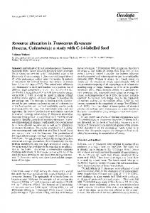
target architecture. The hardware/software partitioning results in a mapping of non-time critical parts of the application to software (i.e. the processor in the target architecture) while the most time critical parts of the application are mapped to the ASIC in order to achieve the software speed-up. As figure 1 shows, the target architecture must be fixed before the partitioning can take place. This includes selecting the processor and allocating the type and number of hardware resources to the hardware data-path (a memory mapped communication scheme between hardware and software is assumed). Specification

Add

ASIC Processor

1 Introduction When designing digital embedded system to be used in cellular phones, laser printers, etc., performance is a critical issue. A well-known technique to meet performance constraints is software speed-up. This is illustrated in figure 1. If the application cannot comply with performance constraints when implemented solely on the processor, time-consuming parts of the application are extracted and executed on dedicated hardware, the ASIC. The target architecture for this type of software speedup is co-processor based, i.e. a single processor and one or more ASICs. This type of target architecture has successfully been used for application speed-up in different co-synthesis systems such as COSYMA [2], Vulcan [3] and the LYCOS system [9]. The ASIC is implemented as a data-path composed of functional units such as adders, multipliers, etc., and a controller that controls the computation in the data-path. This is shown in figure 1, which also shows that the hardware data-path in this target architecture is composed of two adders, one subtractor and one multiplier. We call this an allocation of hardware resources; two adders, one subtractor and one multiplier have been allocated to the hardware data-path. In the LYCOS system, software speed-up is achieved by partitioning the application onto the preselected target architecture using the PACE algorithm [7]. Input to the partitioning tool is the application and the before mentioned

Cont

Datap

Add Sub Mult

Memory

?

HW/SW partitioning

HW/SW mapping

Figure 1. Software speed-up by HW/SW partitioning using a pre-allocated HW data-path

This paper presents a technique that, prior to partitioning, allocates the hardware resources for the hardware data-path. This is a key aspect in the process of achieving the best possible speed-up after the hardware/software partitioning has been done. The preallocation of the data-path resources is done taking characteristics of the application into account, knowing that the application subsequently will be partitioned between hardware and software. The allocations generated by the algorithm comes very close to the optimal allocations. An optimal allocation will ensure that the hardware/software partitioning generated by the PACE algorithm gets maximum speed-up. However, finding the optimal partition for a given application (manually or by exhaustive search) is an extremely time-consuming task due to the very large number of different allocations.

Authorized licensed use limited to: Danmarks Tekniske Informationscenter. Downloaded on June 01,2010 at 12:45:02 UTC from IEEE Xplore. Restrictions apply.

The algorithm is described in the context of the LYCOS system. The algorithm is, however, of a nature that makes it applicable in general. To the authors knowledge, no prior work has been done in the area of allocating resources for hardware while considering the consequences for the combined hardware/software system, although several approaches [1, 4, 5] for allocating resources for an allhardware solution have been proposed. However, in our approach the application is partitioned between software and hardware. The fact that parts of the application will still run as software is taken into account in the hardware resource allocation algorithm.

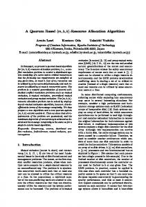
2 The HW resource allocation problem Software speed-up by hardware/software partitioning is in our approach done by dividing the application into appropriate chunks of computation (Basic Scheduling Blocks, BSBs) and then trying out different hardware/software mappings of these. This is illustrated in figure 2A where five BSBs are partitioned onto hardware and software. Moving a BSB to hardware will give the BSB a speed-up. This is due to the fact that in software, operations are executed serially whereas the hardware data-path has multiple resources that can exploit the inherent parallelism between operations in the BSB. B1

B2

Controller area

B3

HW

C

B4

HW Large controller area => room for many BSBs

C

Small controller area => room for fewer BSBs

Data-path area B5

DP

SW

HW

A)

HW-model

B)

Figure 2. Partitioning and HW model

DP

Small datapath => each BSB has a small speedup

A) Many small speedups

Large datapath => each BSB has a large speedup B) Few large speedups

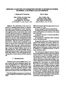
Figure 3. HW allocation tradeoff

The hardware is divided into one piece for the data-path resources, i.e. the functional units that execute the operations in the BSBs, and one piece for the controllers, i.e. the implementations of the finite state-machines that control the execution of the BSBs that are placed in hardware. In our partitioning approach, resources must be allocated to the hardware data-path in advance. The remaining hardware area is the area left for the controllers of the BSBs actually moved to hardware during partitioning. In this way, the cost of moving a BSB to hardware is only the cost of the corresponding controller. This principle is shown in figure 2B, where the two gray boxes indicate the controllers of BSBs B3 and B4, which are moved to hardware by the partitioning algorithm. But allocating the best resources to the hardware data-path is a difficult problem

as illustrated in the following. If the preallocated data-path is small, as in figure 3A, the speed-ups of the individual BSBs are small. However, the small data-path allocation means that there is more room for controllers. As a result, many BSBs may be moved to hardware which leads to many small speedups. If, on the other hand, the data-path allocation is large as in figure 3B, the speed-up of the individual BSBs will be higher since more parallelism can be exploited. However, the large data-path allocation leaves only little room for controllers. Hence, there will be few but large speedups from the BSBs which are moved to hardware. The question is whether the many small speed-ups add up to a higher resulting speed-up than the few large speed-ups? Also, there is the question of which resources should be allocated to the hardware data-path. The discussion above indicates that the preallocation of the hardware data-path resources should somehow balance the requirements for hardware resources against the need for room for controllers while at the same time taking into consideration which types of resources are necessary (e.g. “is an adder necessary?, are two multiplier?, . . . ”).

3

The application model

The applications in our approach are represented as Control Data Flow Graphs, CDFGs. This is illustrated in figure 4. The CDFG is obtained from an input description in VHDL or C. The nodes of the CDFG express loops, conditionals, wait-statements, functional hierarchy and actual computation (the Data Flow Graphs, DFGs). The CDFG is for partitioning purposes translated into a Basic Scheduling Block (BSB) hierarchy. This hierarchy is more suited for partitioning, but contains the same information as the CDFG. The bulk of the application is made up of the leaf BSBs which consist of single DFGs (other BSBs represent the control structures). The leaf BSBs are enclosed by rectangles in figure 4 and they contain the operations (such as multiplication, addition, etc.) that are executed by the BSBs and information about data dependencies between these operations. MAIN

Wait

Body

Test

DFG

DFG

Fu

Loop

Cond

DFG

DFG

Branch1

DFG

CDFG

Wait DFG Loop Test FU

Branch2

DFG

DFG Body DFG Cond Branch1 DFG Branch2 DFG DFG

BSB Hierarchy

B1

B2 B3

B4 B5

Leafs

Figure 4. The CDFG to BSB correspondence

In the allocation algorithm, the application is repre-


sented as an array of leaf BSBs (from now on only denoted BSBs). The application in figure 4 is for example represented by the BSB-array [B1 ; B2 ; B3 ; B4 ; B5 ], corresponding to the BSBs listed to the right in figure 5.

ALLOCATE (BSBArray [1::L]; Restrictions; Area)

f

Allocation, ReqResources, Restrictions : RMap

fg

Allocation RemainingArea Area 1 to L do Move BSBArray[i] to Software for i BSBArray Prioritize(BSBArray) i 1 while ((i L) and (RemainingArea > 0)) AllocationChanged False BSBArray[i] B if (B is in Hardware) then R MostUrgentResource(B) if ((Area(R) RemainingArea) and (Allocation(R) + 1 Restrictions(R)) then Allocation(R) Allocation(R) + 1 RemainingArea RemainingArea - Area(R) AllocationChanged True

4 The hardware resource allocation algorithm The fact that the application in later synthesis stages is going to be partitioned between hardware and software is used in the allocation algorithm. The algorithm generates an allocation by generating a pseudo partition of the application’s BSBs. The basic idea of the algorithm is to try to move as many BSBs as possible to hardware while taking into consideration the hardware cost of moving these BSBs. A BSB has a minimal set of resources required for executing it in hardware (the algorithm considers only the functional resources, i.e. interconnect and storage resources are not considered). When considering moving a BSB, some of these required resources may already have been allocated as a result of other BSBs having previously been moved to hardware. A BSB is moved only when there is room to allocate the (additional) resources and the controller required for executing the BSB in hardware. As a result, an allocation is produced while moving BSBs to hardware. Before describing the algorithm, some basic definitions should be made.

Example 1 Given the two allocations:

Allocation1 : RMap = fAdder ! 2; Multiplier ! 1g Allocation2 : RMap = fSubtractor ! 1; Multiplier ! 2g

the operators [ and n will result in e.g.:

Allocation1 [ Allocation2 = fAdder ! 2; Multiplier ! 3; Subtractor ! 1g Allocation1 n Allocation2 = fAdder ! 2g Allocation2 n Allocation1 = fSubtractor ! 1; Multiplier ! 1g Indexing and updating in RMaps results in e.g.:

Allocation1(Adder) + 1 = fAdder ! 3; Multiplier ! 1g The algorithm is shown in algorithm 1. Before entering the main loop, the array of BSBs is prioritized, see section 4.1. Then, starting with the first BSB in the prioritized array, if it is already in hardware, some operation in the BSB is urgent and, if possible, one more resource that can execute this operation should be allocated (the name of the

f

g g else f

n

ReqResources GetReqResources(B) Allocation ECA(B) + Area(ReqResources) Cost if (Cost RemainingArea) then Allocation Allocation ReqResources RemainingArea - Cost RemainingArea Move BSBArray[i] to HW AllocationChanged (ReqResources = )

g

[

f

6 fg

g

f

if (AllocationChanged) then BSBArray Update (BSBArray, Allocation) BSBArray Prioritize(BSBArray) i 1 else i i+1

g

RMap Resource ! Integer

[ : RMap RMap ! RMap n : RMap RMap ! RMap

f

f

Definition 1 Define the following type:

An RMap (Resource Map) is a mapping from resources to integers. Two operators are defined on RMaps:

g g

return Allocation

Algorithm 1. The hardware allocation algorithm

resource is returned by the function MostUrgentResource). If this is possible (if the area of the resource is less than the remaining hardware area, and the restrictions are not violated, see section 4.3), the allocation and the remaining area are updated. If the allocation of the required resource is not possible, the BSB is skipped. If the BSB currently being investigated is still in software it should be tried to move it to hardware. Moving a BSB to hardware will induce a cost (see section 4.2), which consists of the Estimated Controller Cost (ECA) and the cost of allocating (additional) resources in order to execute the BSB in hardware. These additional resources are the resources in ReqResources which equal the resources necessary to execute the BSB in hardware (found by the function GetReqResources) minus the already allocated resources.


After investigating the current BSB, B, the allocation might have changed as a result of allocating one more resource for an operation in B (if B was already placed in hardware) or as a result of moving B from software to hardware. If the investigation of B has resulted in a new allocation, the information associated with each BSB is updated, see section 4.1, and the array is re-prioritized. If not, B is skipped and the next BSB in the array is investigated. If the last BSB is reached without having changed the allocation, or if the remaining area reaches zero, it means that no more BSBs can be moved to hardware and no more resources can be allocated; the algorithm exits and returns the obtained allocation.

4.1

Prioritizing the BSBs

When considering which BSBs to move to hardware, a metric of urgency is employed when prioritizing the BSBs. Consider a BSB in the application. Each operation in the BSB will, if the BSB is placed in hardware, be executed by some resource in the hardware data-path. If the BSB contains a lot of operations of a specific type, and the number of resources that can execute this type of operation is small, the final hardware schedule produced during the hardware/software partitioning process will be stretched, leading to a loss of performance. Note that the communication overhead of moving a BSB to hardware is ignored. This is due to the fact that the algorithm works at an early stage in the design flow, using a limited amount of information about the application. At this point in the design trajectory the main issue is to get a good guess on a feasible hardware data-path allocation fast, thus it is acceptable no neglect certain characteristics such as the communication overhead. If too many characteristics are taken into account, the algorithm would become too slow. Since hardware is able to exploit the inherent parallelism between operations in a BSB, BSBs with heavy inherent parallelism are prioritized over BSBs which do not have as heavy inherent parallelism. However, since the total execution time of a BSB is also determined by the number of times it is executed (during one execution of the application), the priority function is also based on profiling information. The algorithm is guided towards allocating resources for operations that can be executed in parallel. As an estimate of the inherent parallelism in a BSB, the Functional Unit Request Overlap (FURO), which estimates the probability that two operations in a BSB will compete for a hardware data-path resource, is used. The estimate is an extension of the one in [10]:

Definition 2 Let i and j be operations in a BSB, Bk , and let pk be the profile count for Bk . The Functional Unit Request Overlap, FURO, for the operation of type o in Bk is:

FURO(o; B ) = p k

k

P

Ovl(i;j )

i;j;i6=j M (i)M (j )

0;

; T (i) = T (j ) = o ^j 2= Succ(i) î 2= Succ(j ) otherwise

T(i) returns the type of the operation i, Ovl(i,j) is the overlap of the ASAP-ALAP intervals of the two operations and M(i), M(j), respectively, is the mobility of the operation (ALAP - ASAP + 1). In figure 5, M(i) = 5 - 1 + 1 = 5, Ovl(i,j) = 3. Note, that it is necessary to ensure, that the two operations are not successors of each other, since if they are, they cannot compete for resources, since they cannot be scheduled in the same control-step (Succ(i) returns the set of all successor operations of i).

t=1

i j

t=2 t=3

j

t=4 t=5

i

Figure 5. Overlap of operations

The higher the overlap is, the higher is the probability that the two operations will be scheduled in the same control-step. On the other hand, if the operations have large mobilities, they could probably be moved away from each other in the final schedule. Each BSB Bk is for each operation o annotated with a value U (o; Bk ). Definition 3 Let o be an operation type and Bk a BSB. Let InHW(Bk ) be the function that returns true if Bk is in hardware, false otherwise. Then

U (o; B ) = FURO(o; B ); if not InHW(B (o; B ) U (o; B ) = FURO Alloc(o) + 1 ; if InHW(B ) k

k

k

k

k

)

k

Alloc(o) returns the number of resources allocated so far, that can execute an operation of type o. In this way, as the allocation grows, U (o; Bk ) will decrease for a given BSB Bk placed in hardware and a given operation o. The priority of BSBs is based on the values U (o; Bk ): Definition 4 Let Bk Bl . Then

B !B k

l

! Bl mean that Bk has priority over

, max(U (o1 ; B )) max(U (o2 ; B )) k

l

for all operation types o1 ; o2 (if a BSB, Bk , does not have operations of type o, U (o; Bk ) is zero).


This means, that when considering two BSBs, the BSB with the highest U (o; Bk ) for any type of operation o will have priority over the other, meaning either that the BSB should be moved to hardware before the other BSB or, if it is already in hardware, contains an operation o for which it is urgent to allocate one more resource before it can be considered to move the other BSB to hardware. Example 2 Consider two blocks B1 and B2 which, for the sake of simplicity, contain only one operation type denoted o0 . At first, B1 is prioritized over B2 because U (o0 ; B1 ) U (o0 ; B2 ). Then B1 is moved 0to hardware, and a resource that can execute operation o is added to the allocation (if one was not allocated already). Now, according to definition 3, U (o0 ; B1 ) drops while U (o0 ; B2 ) stays the same because B2 is still in software. As long as U (o0 ; B1 ) U (o0 ; B2 ), resources that can execute o0 are added to the allocation, but in this way, B2 could get priority over B1 and as a result also be moved to hardware. As shown in example 2, BSBs that already benefit from being placed in hardware are dynamically given lower priorities than BSBs still in software. The updating of the information associated with the BSBs mentioned in section 4 means re-calculating the values U (o; Bk ) as a result of allocating additional resources.

4.2

The cost of moving a BSB

The algorithm starts with all BSBs being placed in software. Moving a BSB to hardware will induce a cost in terms of hardware area. Part of this area is the controller area, part is the area of the allocation of resources necessary to execute the BSB in hardware. The controller is composed of a number of registers to hold the state. The number of states for a BSB is estimated as the ASAP schedule length. This estimate is optimistic, but it is the only estimate available, since there is no allocation available to generate a more precise listbased schedule (the allocation is what we are looking for). The number of registers necessary to hold the states for a BSB is proportional to log2 (N ) where N is the estimated number of states of the BSB. In addition, the controller has decode logic which is proportional to N . In all this means that the control logic is proportional to log2 (N ) + N . A more thorough description of the controller size estimate can be found in [6], where it is shown that the Estimated Controller Area, ECA, is calculated as

AR + AAG + AOG + log2(N ) AR + (N , 1) (AIG + 2 AAG ) where AR ,AAG ,AOG , and AIG are the areas of a register, ECA

=

an and-gate, an or-gate and an inverter-gate. The other part of the cost of moving a BSB to hardware is the total area of the resources necessary to execute the operations of the BSB. The algorithm will, when

a BSB is moved to hardware, allocate a minimum of resources (maximum one of each) so that all operations in the BSB can be executed. Note, that the allocation might in advance contain resources that can execute some of the operations in the BSB. This means that the new resources are added to the existing allocation only if they are necessary. For instance, if the BSB that should be moved to hardware contains only additions and multiplications, and a subtracter and a multiplier has already been allocated, the only required resource for moving this BSB to hardware is an adder. The total cost of moving a BSB from software to hardware can now be formulated as:

Cost 4.3

=

ECA + Area(RequiredResources)

Allocation restrictions

Since the allocation algorithm is greedy, a situation where it allocates too many resources that can execute a specific operation type can occur. The ASAP-schedule can be used to give an estimate of the maximum number of operations of a specific type that can be executed in parallel. The algorithm will not produce allocations that exceed these limits (a maximum of 3 multipliers, for instance).

4.4

Algorithm complexity

The runtime of the allocation algorithm is difficult to estimate. However, the runtime of the initial computation of the Functional Unit Request Overlaps is proportional to L k2 , where L is the number of BSBs and k is the maximum number of operations in any of the BSBs. It is the computation of the FUROs that is the time consuming task, but this computation is only done once. The allocation algorithm could be executed several times for the same array of BSBs with different area constraints, different hardware resource library (or restrictions for that matter).

5

Results

The quality of the allocations generated by the allocation algorithm is evaluated using the PACE algorithm [7]. First, the PACE algorithm is used to generate a partition of the application for all possible allocations. Through this exhaustive search, the allocation that gives the best partitioning result in terms of speed-up is marked as the best allocation. The PACE algorithm is then used to generate a partition using the allocation generated by the allocation algorithm, and this result is compared with the partitioning result obtained with the best allocation. Four applications have been used to test the allocation algorithm, and the results after partitioning are shown in the table below. The table shows the size of the applications and the speed-up that can be achieved using the allocation found by the algorithm compared with the speed-up (SU) that can be achieved using the best allocation (speedup is computed as the decrease in execution time from


an all software solution to a combined hardware/software solution including hardware/software communication time estimates). The column Size shows the size of the allocation (i.e. HW data-path) in percentage of the total size of the HW data-path and controllers (interconnect and storage are ignored in these figures). The next column shows how much of the applications were placed in HW and how much in SW, and the last column shows the run-time for the allocation algorithm on a Sparc20. hal is the well-known example from [11], man is an application that calculates the Mandelbrot set [12] and eigen is an algorithm that calculates the eigen-vectors in an algorithm that computes interpolated cloud-movement pictures for a stream of meteo-satellite pictures [8]. straight is taken from [9]. Example straight hal man eigen

Lines 146 61 103 488

SU/SU(best) 1610%/1610% 4173%/4173% 30%/3081% 20%/311 %

Size 62% 93% 92% 82%

HW/SW 58%/42% 80%/20% 8%/92% 19%/81%

CPU sec 0.1 0.2 0.2 0.5

Table 1. Results

The explanation of the third result, which apparently looks quite bad, is that the application contains a lot of parallel loading of constant values for multiplication. These constant loadings are situated in a single BSB which means that the estimated number of states, N , and hence the ECA is extremely poor for this block when moved to hardware. Therefore, the algorithm allocates many constant generators which reduces the available controller area, and therefore the partitioning algorithm cannot move as many BSBs to hardware. However, with a single design iteration, in which the number of allocated constant generators was reduced from the automatically generated value to a value of one, the Best SU was obtained. The same was the case for the eigen example; one design iteration where only the number of allocated resources that executes division was reduced by one was necessary to obtain the Best SU solution. It might seem strange that a speed-up of 3081% can be achieved for the Mandelbrot example by placing only 8% of the application in HW. However, these 8% constitutes an extremely computing intensive part of the algorithm. Thus a large speed-up can be achieved by placing this fraction of the application in HW.

5.1

The effect of optimistic controller estimation

In section 4.2 it was shown how the controller is estimated on basis of an ASAP schedule length. This is of 1 The eigen benchmark has approximately 1.000.000 different allocations. Evaluating one allocation takes more than 30 seconds which makes exhaustive evaluation impossible. The allocation which makes the best speed-up is the best allocation found using numerous experiments from tutorial sessions with the LYCOS environment.

course an optimistic estimate of the final schedule length – the resulting controllers for BSBs actually moved to hardware are larger. This means that the algorithm will allocate a few too many resources for the hardware data-path than actually affordable. However, knowing this, the designer can always reduce the number of allocated resources slightly in order to obtain the best possible partitions. It is never necessary to increase the number of allocated resources to achieve the best allocation.

6

Conclusion and future work

This paper has presented a novel allocation algorithm for hardware/software partitioning which allocates resources to the hardware data-path. The allocations generated come close to the best possible allocations obtained exhaustive search. Directions for future work includes extending the algorithm to be able to deal with selection between several resources that can execute the same type of operation. Another extension is the generalization to target architectures that contain more than one ASIC. Also, aspects such as incorporating interconnect and storage size estimates would be interesting to look into.

References [1] S. Devadas and A. R. Newton. Algorithms for Hardware Allocation in Data Path Synthesis. IEEE Transactions on CAD, 8(7):768–781, 1989. [2] R. Ernst, J. Henkel, and T. Benner. Hardware/Software CoSynthesis of Microcontrollers. Design and Test of Computers, pages 64–75, Dec. 1992. [3] R. Gupta. Co-Synthesis of Hardware and Software for Digital Embedded Systems. Kluwer Academic Publisher, 1995. [4] P. Gutberlet, J. Müller, H. Krämer, and W. Rosenstiel. Automatic Module Allocation in High Level Synthesis. In EURODAC, pages 328–333, 1992. [5] R. Jain, A. Parker, and N. Park. Module Selection for Pipelined Synthesis. In 25th ACM/IEEE DAC, pages 542– 547, 1988. [6] P. V. Knudsen. Fine Grain Partitioning in Hardware/Software Codesign. Master’s thesis, Technical University of Denmark, 1996. [7] P. V. Knudsen and J. Madsen. PACE: A Dynamic Programming Algorithm for Hardware/Software Partitioning. In 4th Int’l Workshop on Hardware/Software Codesign, pages 85 – 92, 1996. [8] R. Larsen. Estimation of Visula Motion in Image Sequences. PhD thesis, Technical University of Denmark, 1994. [9] J. Madsen, J. Grode, P. V. Knudsen, M. E. Petersen, and A. E. Haxthausen. LYCOS: the Lyngby Co-Synthesis System. Design Automation for Embedded Systems, 2(2), April 1997. [10] Miodrag Potkonjak and Jan Rabaey. Optimizing Resource Utilization Using Transformations. IEEE Transactions on CAD of ICs and Systems, 13(3):277–292, March 1994. [11] P. G. Paulin and J. P. Knight. Force-Directed Scheduling for Behavioral Synthesis of ASICs. IEEE Transactions on Computer-Aided Design, 8(6):661 – 679, June 1989. [12] H.-O. Peitgen and P. Richter. The Beauty of Fractals. Springer-Verlag, 1986.
