Haskell#: Parallel Programming Made Simple and ... - Semantic Scholar

Haskell# : Parallel Programming Made Simple and Efficient Francisco Heron de Carvalho Junior1∗, Rafael Dueire Lins2† 1 2

Centro de Inform´atica

Departamento de Eletrˆonica e Sistemas

Universidade Federal de Pernambuco, Recife, Brazil [email protected], [email protected]

Abstract. This paper presents the final result of the designing efforts for the development of a new specification for the Haskell# Language, including new features to increase its expressiveness, but without losing neither efficiency nor obedience to its original premisses.

1. Introduction Haskell# is an explicit parallel distributed language, defined on top of Haskell, that has evolved since 1998[Lima and Lins, 1998]. The premisses that guide its design attempt to make parallel programming a task reachable for most programmers, without have to pay for loss of efficiency of parallel programs when running over distributed architectures, such as clusters[Baker et al., 1999]. Below, we discuss them: • Ideally, parallelism would be implicit, freeing programmers from the burden of control communication and synchronization concerns. However, practice has demonstrated that efficient implicit parallelism is hard to obtain in its general case, due to the high complexity of the configuration tasks required to parallelise sequential programs, such as partitioning, allocation, granularity control, and so on. To parallelise efficiently, compilers should take into account many concerns about intrinsic features of the target archicteture and the application. This is not always easy to model. Even in functional languages, where parallelism is easier to detect, the results obtained are very poor, if compared to explicit approaches [Loidl et al., 2000]; • Dynamic control of parallelism, involving tasks such as process migration for load balancing processors and on demand creation of processes, generates a high overhead in the run-time of parallel programs, increasing proportionally to the communication latency amongst processors of the target distributed architecture; • In paralell programs, the interleaving of the primitives for control of parallelism and the computation code makes the analysis of formal properties very hard. This way, it is impossible to abstract process interaction from computation; ∗ †

Supported by CAPES. Supported by CNPq.

• The mixture of computation and parallelism control code also difficults programming, requiring skilled and well trained parallel programmers, increasing the costs of the development of complex parallel applications; • The lack of a unified and consensual model for parallel programming lessens portability and existence of systematic parallel development methods and tools. The intimate relationship between existing programming models and parallel archictectures serves to explain the diversity of the first ones[Skilikorn and Talia, 1998]. Haskell# was designed based on the above assumptions. Thus, it now supports the following features: • Explicit and static paralellism configuration. For minimizing overheads in the execution time of parallel programs, assuming that the programmer is the most capable specialist to perform the configuration of parallel tasks efficiently, due to his/her knowledge about target archictecture and the application and the inexistence of efficient algorithms to perform optimally configuration tasks in their general instances automatically; • Efficient and simple implementation. Haskell# only requires to “glue” a Haskell sequential compiler to a message passing library. GHC and MPI, respectively, have been used in this work. The use of an efficient sequential Haskell compiler is important, assuming that Haskell# style of programming encourages coarse grained parallelism, where most of time is expended in performing sequential computations; • Abstraction of parallelism from computation. In essence, Haskell# encompasses a coordination language[Gelernter and Carriero, 1992, Carvalho Jr. et al., 2002a]. Computations (Functional Processes) are described in Haskell, while coordination (parallelism configuration) is described by means of HCL (Haskell# Configuration Language). HCL is synthatically orthogonal to Haskell. No extensions or libraries are necessary to Haskell for gluing processes to coordination medium, described in HCL. This characteristic induces a process hierarchy, with several benefits, such as higher degree of modularity, in many aspects of programming, and simplication of programming task; • Equivalence to Petri Nets. HCL descriptions can be translated into (labeled) Petri nets[Petri, 1966] that describes the process interaction and communication behaviour of parallel programs, making possible effective formal properties analysis about them[Carvalho Jr. et al., 2002b]; • Hierarchical Compositional Programming. Compositional programming is an important technique to increase the modularity of programming languages, most specially in parallel ones [Foster, 1985]. Hierarchical composition is an important feature supported by modern configuration languages in distributed systems[Krammer, 1994, Magee et al., 1995]. It adds to Haskell# new abstraction mechanisms for describing complex network topologies in a simple way; • Partial Topological Skeletons. Skeletons are an important programming technique developed by Murray Cole in eighties[Cole, 1989]. They allow to orthogonalise the description of an algorithm from its efficient implementation in a specific architecture. General reusable patterns of process interaction found in concurrent programs define a skeleton. Haskell# partial topological skeletons

makes easier to describe complex network topologies, giving support for nesting and overlapping operations to allow composition of skeletons from existing ones[Carvalho Jr., 2003]. Tree other sections compose this paper. Section 2. briefly explains the evolution of Haskell# since its original conception. Section 3. describes the structure of Haskell# programs, and also presents some representative examples. Finally, Section 4. draws some conclusions and lines for current and further works in Haskell# .

2. The Evolution of Haskell# Since its first publication four years ago [Lima and Lins, 1998], three versions of Haskell# language have appeared. Each version has tried to improve the previous one in meeting the targets described in Section 1. of this paper. In the first Haskell# version [Lima et al., 1999], funcional processes communicated by making explicit calls to message passing primitives defined on top of Haskell IO monad. HCL was used to define the communication topology of processes, connected via OCCAM-style channels. The use of explicit message passing primitives extending Haskell, allowing mixture of parallelism synchronization primitives with computational code, broke Haskell# principle of process hierarchy, making impossible automatic analysis of formal properties of programs with Petri nets. The inference of communication behaviour of processes was impossible by automatic means. The first revision of Haskell# produced a new version, where explicit message passing primitives were abolished in favor of process hierarchy. Communication input and output ports of functional processes became mapped onto arguments and elements of the tuple returned by their main functions, respectively. Ports are connected to define communication channels, as in the first version. Functional Processes were strict, which means that values should be transmitted in their normal forms. A process is executed by performing the following tasks in sequence: read input ports in the order in which they were declared in the HCL program; call the main function, giving to it, as arguments, the values received by input ports, in the order they were received; send each element of the returned tuple, by function main, through output ports, in the order they were declared. Not allowing functional processes to perform communication interleaved with computation turned difficult to express important concurrency process interaction patterns used in some parallel applications, such as systolic and pipe-line computations. These applications require that processes exchange information while they compute, or keep state between communication operations during computation. However, this version allowed us to define the first translation of Haskell# programs into Petri nets and to analyse communication behaviour of some applications, such as an ABS (Anti-Braking System) control unit [Lima and Lins, 2000]. This was very important to demonstrate the potential of Haskell# approach for parallel programming. The lastest version of Haskell# was developed to concile maximal concurrency expressiveness with process hierarchy and also to provide higher abstraction programming mechanisms without ANY loss of efficiency. Special attention has been dedicated to translation into Petri nets. Lazy stream communication was introduced to allow a process to interact during computation. Viewed from functional processes, lazy streams are

Distributor

mA mB

farmA farmB

Workers Collector

mm’s mm’s

mC mC

mA mm[1][n]

mm[2][1]

mm[2][2]

...

mm[2][n]

...

mm[m][n]

mm[m][1]

mm[m][2]

...

...

...

mm[1][2]

...

mm[1][1]

mC

mB

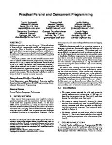
mm[i][j] = matmult[i][j] Figure 1: Matrix Multiplication Topology

essencially Haskell lazy lists, whose elements can be read or written on demand. This characteristic allowed to abstract communication operations from computation in programming, but without loss of the ability to allow processes to interact dynamically. Ports now can be read on demand. The support for skeletons and hierachical compositional programming allow for a more abstract and higher-level style of programming. This version of Haskell# is described in the following sections.

3. The Structure of Haskell# Programs This section describes the structure of Haskell# programs, concentrating on their logic structure, but illustrating syntatic aspects by means of examples. The main example used here is a Haskell# implementation for a very well known systolic algorithm for matrix multiplication, described in [Manber, 1999]. It allows to demonstrate important aspects of Haskell# programming, such as the use of skeletons, hierarchical composition, and so on. The implementation of the matrix multiplication follows the network structure presented in Figure 1. Two processes, named mA and mB read and distributes matrixes to be multiplied by a collection of matmul processes organized in a mesh. The indexes that identifies individually these processes indicates its position (line and colunm) in the mesh. A process mC is responsible for receiving the result of the multiplication and presenting it to the user. The skeletons FARM and MESH are used to compose this network topology. Figures 2 and 3 present the HCL code for a Matrix Multiplication component, and the functional module Haskell code for the cooperating processes that perform multiplication, repectively.

– In File matrix multiplication.hcl component MatrixMultiplication with index i, j range [1,N] use module MatrixMultiplication.MatMult use module MatrixMultiplication.ReadMatrix use module MatrixMultiplication.ShowMatrix use configuration Skeletons.Common.FARM use configuration Skeletons.Common.MESH interface MatMul (a, b, l, u::MMData) → (r, d, c::MMData) behaving as SystolicMeshCell # (l,u) → (r,d) as seq { par {read a; read b}; repeat seq {write r; write d; read l; read u} until count N; write c } unit mA as ReadMatrix N → out # Distributor () → out*N*N:partition by DistMatrix::MMData unit mB as ReadMatrix N → out # Distributor () → out*N*N:partition by DistMatrix::MMData unit mC as ShowMatrix # Collector in*N*N:combine by CollMatrix::MMData → () unit farmA as FARM unit farmB as FARM unit mmgridas MESH [/ unify farmA.worker[(i+1)*N + j] # a → c, farmB.worker[(i+1)*N + j] # b → c, mmgrid.meshcell[i][j] # (l,u) → (r,d) to matmult[i][j] as MatMult (N,a,b,l,u) → (r,d,c)# MatMul (a,b,l,u) → (r,d,c) /] unify mmfarmA.collector # c → (), mmfarmB.collector # c → () to showmatrix # c → () assign mA to mmfarmA.distributor assign mB to mmfarmB.distributor assign mC to showmatrix Figure 2: HCL code for a matrix multiplication on a circular mesh

– In File matmul.hs module MatMult(main) where main :: Int → Int → Int → [Int] → [Int] → IO (Int, [Int],[Int]) main n aij bij as bs = return (matmul (aij*bij) n aij bij as bs) matmul :: Int → Int → Int → Int → [Int] → [Int] → (Int, [Int], [Int]) = (c,[],[]) matmul c 1 matmul c n aij bij (a:as) (b:bs) = (cij,aij:as’,bij:bs’) where (cij,as’,bs’) = matmul (c+a*b) (n-1) a b as bs Figure 3: A functional module for processes matmul in Matrix Multiplication

3.1. Units: The Building Blocks of Haskell# Programs A Haskell# application is structured as a tree, where nodes are units, abstractions for executing entities. The unit at the root is called main unit, because it defines the computation of the program. An interface and a component should be associated with a unit. 3.1.1. Interfaces: Describing How Units Interact An interface defines the set of input and output ports of the unit, from which they communicate with other, as well as the order in which they are activated (communication behaviour). The order is defined by an expression written in a OCCAM-like[Inmos, 1984] language, designed in such way that its expressive power is equivalent to expressive power of labeled Petri nets. The HCL piece of code below defines an interface: interface SystolicMeshCell (left*, top*::[t]) → (right*, bottom*::[t]) behaving as Pipe # left → right as Pipe # top → bottom as repeat par {left; top; right; bottom} until (left, top)

The interface SystolicMeshCell has two input ports, named left and top, and two output ports, named right and bottom. All ports are lists of some unknown type (polymorphism). The * after the name of each port means that the list typed port must be treated as a lazy stream, whose elements are received or sent one at a time. The behaving clause introduces behaviour constraints. In the example, SystolicMeshCell has three behaviour constraints. The first two says that a systolic mesh cell must behave like a pipe-line stage, when considering ports left and right, or ports top and bottom, making the hole of in and out ports of a pipe-line stage, respectively. The last constraint describe the communication behaviour for the interface. The compiler has to check its compability with other behaviour constraints, producing an error message whenever necessary. An interface can have many behaviour restrictions (like the first two in the example above), but only one is a communication behaviour. If the programmer does not define a communication behaviour code, the compiler will derive one automatically, which is the weakest communication behaviour that satisfies the other behaviour constraints, if they exist. 3.1.2. Components: Describing What Units Compute A component defines the computation performed by the unit and can be simple or compound. Simple components are Haskell programs, called functional modules, that are the primitive and effective computational entities of Haskell# programs. Units instantiated from simple components are called processes. Compound components are HCL configurations, defining a network of cooperating units. Units instantiated from compound components are called clusters. Programs in Figure 2 and 3 illustrate a compound component declaration (HCL configuration) and a functional module, respectively. In the compound component MatrixMultiplication, the parameter @N defines the dimension of the matrices. The following declarations configure the functional process network, whose diagram is shown in

Figure 1. In the functional module MatrixMult, one may observe that there are no extensions or special libraries introduced in the Haskell code, due to the orthogonality between HCL and Haskell.

expr::t

ignored value

a

module Example(main) where

2

expr

main :: t −> u −> v −. IO (r, s, q) main x y z = ... return (v,w) ignored value

Process

Cluster

Figure 4: Entry and Exit Points

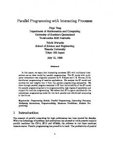
Components may have entry and exit points, which are mapped to input and output ports of the unit, respectively. For functional modules, entry points are the arguments of the function main, while exit points are the elements of the tuple returned in the resulting IO action. For HCL configurations, entry and exit points are bound to input and output ports, respectively, that are not connected by any channel. Entry and exit points are illustrated in Figure 4. In the compound component declared in Figure 10, one entry point and one exit point are declared, respectively named in and out. The bind declaration at the end of the HCL configuration declares that the input and ouput ports are bound to the mentioned entry and exit points. In the hierarchical view of any Haskell# program, instantiated in Figure 5, the units at the leaves are processes, while internal units are clusters. The units that have the same parent node belong to the same HCL configuration.

Main Unit Simple Component Composed Component

Units Functional Process Cluster

Figure 5: Unit Hierarchy in a Haskell# Program

3.1.3. Repetitive and Non-Repetitive Units There are two kinds of processes: non-repetitive and repetitive. The former ones reach final state after evaluate function main, while the latter ones may execute forever, by calling repeatedly and sequentially its function main. A cluster is said to be repetitive if all units that compose it are repetitive. The compiler generates an error message if the programmer attempts to declare as non-repetitive a cluster where all composing unit are repetitive. A Haskell# program that has as main unit a repetitive unit is said to be repetitive. Repetitive applications are very useful to implement reactive applications, programs which do not reach a final state. In general, those are systems that interact with the environment, like operating or control systems. An example of a declaration of a repetitive unit is shown below: unit * random as Random # seed → number

The * symbol after the keyword denotes that the unit random is repetitive. Each time the unit (process) random is activated, a random number is generated according to a seed value.

3.1.4. How to Declare a Unit The HCL declaration below defines many units in a single line, using indexed notation of HCL: index i, j range [1,N] .. . [/ unit grid cols[i] as PIPE-LINE in → out # Pipe in → out /]

The index declaration specify two indexes, whose range is configured in range clause, from 1 to N, where N is a configuration parameter. The delimiters [/ and /] delimits a scope for varying indexes declared inside. In the example, notice that i is the index that is in the scope of the delimiters. N units are declared, named grid cols, and distinguished by indexes from 1 to N. The grid cols units are instances of the compound component PIPELINE, forming clusters. Its interface is Pipe, defining one input port, named in and an output port, named out. Observe that the entry and exit points of PIPE-LINE component are mapped onto input and output interface ports of the unit by matching identifiers. In the declaration of a toroidal mesh skeleton (Figure 9), the ports in and out of grid cols clusters will be connected to define circular pipe-lines.

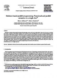
3.1.5. Replication of Ports in Unit Declarations When defining the interface of a unit, the programmer can replicate ports of the interface to define groups of ports, controlled by the protocols whose semantics is described in Figure 6. The protocols at the top (partition, broadcast, and choice) are for input ports, while that at the bottom (combine, merge, and choice) are for output ports. The protocols partition and combine require definition of partition and combination strategies, respectively. They define Haskell functions used to partition or combine values of the group

Broadcast

v

v1 v2

v

v

...

v

partition v =[v1,v2,...,vn]

Merge

Combine v1 v2

v1 v2

v

Choice

[v1,v2,...vn]

vn

v

v

...

vn

...

...

Input

v v

...

vn

v

Choice

...

Output

Partition

v = combine [v1,v2,...,vn]

Waiting Port

Entry point (ti)

Prepared port

Exit Point (ui)

Component

Figure 6: Group of Ports Protocols

of ports data type. In Figure 2, the reader can see how groups of ports are declared, in interface specification of units mA, mB and mC. 3.2. Communication Channels Haskell# communication channels are used to connect ports of opposite directions from two processes. They are synchronous, point-to-point, unidirectional and typed. In this new Haskell# version, bounded buffers were introduced for allowing a weak form of assynchronous communication. The declaration below illustrates the syntax of a channel declaration in HCL : index i, j range [1,N] .. . [/ connect * grid cols[i].pipe[N]→out to grid cols[i].pipe[1]←in buffered 10 /]

In the example above, N channels are declared. Let v an index value (value of i), the channel links the port pipe[@N] of unit grid cols[v] to the port pipe[1] of the same unit. The * after the connect combinator indicates that the channel transmits a stream. The ports connected by a stream channel must be declared to be streams too, or the compiler will generate an error message. The clause buffered is facultative and stabilishes a buffered channel. The buffer size is configured as an integer value after buffered clause. In the example, its value is 10. If ommited, the buffer size is assumed to be limited to the amount of available memory. 3.3. Virtual Units: Towards Skeleton Programming It is possible to define a unit without a component, but an interface is always required. When an interface is not provided, a default one is implicitly assumed. A unit for which a component does not exist is called a virtual unit (Figure 7). Virtual units are essentially templates from which non-virtual units can be defined. At any moment, a non-virtual component can be assigned to a virtual unit, occupying its place and assuming its role in the network of units. For that, there must be a behavior constraint that associates the interface of the assigned unit to the interface of the virtual unit. Remember that behavior constraints were discussed in Section 3.1.1.

(non virtual) unit

virtual unit

interface

interface

component

?

Figure 7: Virtual and non-virtual

The syntax for declaration of virtual units can be observed in Figures 8 and 9. It is similar to a non-virtual unit declaration, but the virtual keyword is used before the unit keyword. The clause as, used to define the component, is not necessary. An example of use of assignment operation is presented in Figure 2. The process mA is assigned to the virtual unit distributor of the cluster mmFarmA. In the declaration of process mA, observe that it is configured to be the interface Distributor, the same of the virtual unit distributor, allowing compiler to perform the appropriate assignment. The compound component in Figures 8, 9, and 10 are called skeletons, once they define virtual units in their compositions. FARM, MESH and PIPE-LINE are three of the most common skeletons. Others are HYPERCUBE and TREE, omitted due to space restrictions. Skeletons are a important programming technique introduced by Murray Cole in 80’s[Cole, 1989]. – In file farm.hcl component FARM with export interface Distributor, Worker, Collector interface Distributor () → out behaving as repeat write out until out interface Worker in → out behaving as repeat read in until in interface Collector in → () behaving as repeat read in until in virtual unit distributor # Distributor () → out virtual unit worker # Worker in → out virtual unit collector # Collector in → () connect distributor→out to worker←in connect worker→out to collector←in replicate N worker # in → out connections in: partition, out: combine Figure 8: FARM Skeleton

The skeletons mentioned here are examples of total skeletons, because all computational entities are parameterized, a widely adopted assumption. Haskell# also allows for partial skeletons, where some of the computational entities (units) are completely defined.

– In file mesh.hcl component MESH with use configuration Skeletons.Common.PIPE-LINE export interface SystolicMesh index i, j range [1,@N] interface SystolicMeshCell (left*, top*::[t]) → (right*, bottom*::[t]) behaving as Pipe # left → right as Pipe # top → bottom as repeat par {left; top; right; bottom} until (left, top) [/unit grid cols[i] as PIPE-LINE # in → out/] [/unit grid rows[i] as PIPE-LINE # in → out/] [/connect * grid cols[i].pipe[N]→out to grid cols[i].pipe[1]←in/] [/connect * grid rows[i].pipe[N]→out to grid rows[i].pipe[1]←in/] [/unify grid cols[i].pipe[j] # l → r, grid rows[j].pipe[i] # t → b to cell[i][j] # SystolicMeshCell (l,t) → (r,b)/] Figure 9: MESH Skeleton

3.3.1. Unification and Factorization of Virtual Units Two operations can be performed with virtual units: unification and factorization. The former allows for programmers to compose new virtual units from a set of virtual units, by composing them. The interface of the new virtual unit assumes behavioral constraints that relates it to the interfaces of the original units. This means that the new unit must preserve the behavior of the original units in the network. Factorization is the dual of unification, allowing for a unit to be divided into two or more units, preserving the behavior of the original units, by applying the restrictions of its interface. An example of unification is demonstrated in the HCL code for the MESH skeleton component in Figure 9. The units that compose the N grid cols pipe-line units and N grid rows pipe-line units are unified in a mesh. This is an example of overlapping of skeletons, which can be used to compose a new skeleton as demonstrated in the presented example. Another way to compose new skeletons from existing ones is nesting, where a skeleton unit is assigned to a virtual unit of another skeleton. 3.4. Replication of Units: The Essence of Distributed Data Parallel Computations An operation is defined over any kind of units: replication. It allows to construct many copies of an unit in the network. Amongst other uses, replication is suitable to define distributed data-parallel computations. An example of replication is shown in FARM skeleton declaration in Figure 8. An unit named worker is defined and then replicated to form the set of farm worker processes, indexed from 1 to N. Special attention must be given to the ports connected to the replicated process. They must be also replicated, in such way that now there is a copy of the original port for each unit derived from repli-

– In File pipe.hcl component PIPE-LINE in → out with export interface Pipe index i range [1,N-1] index j range [1,N] interface Pipe in* → out* behaving as repeat seq{read in; write out} until in [/virtual unit pipe[j] # Pipe in → out;/] [/channel link[i] connect * pipe[i]→out to pipe[i+1]←in/] bind pipe[1]←in to in bind pipe[N]→out to out Figure 10: PIPE Skeleton

cation. Notice that, in the example, the resulting groups of ports of units distributor and collector are controlled by partition and combining protocols, but the strategies are not specified. When assigning non-virtual units to FARM virtual ones, the programmer should define these strategies, configuring the FARM according to his needs. An example of this approach can be seen in the matrix multiplication HCL code 2, where strategies (DistMatrix and CollMatrix) makes the role of distribution and combining strategies of FARM’s f armA and f armB after assignment of mA, mB and mC to their virtual units. 3.5. Startup Modules: Putting Things to Work Startup modules defines the main unit of the application, giving, whenever necessary, values to be passed to its entry ports. If the main unit have output ports, the values produced by them at the end of computation can be given to an exit Haskell function, which perform some final computation with the yielded values. The startup module for the matrix multiplication program is presented in Figure 11. application MatrixMultiplication with use configuration MatrixMultiplication.MatrixMultiplication unit main as MatrixMultiplication Figure 11: Matrix Multiplication Startup Module

The example below demonstrates full functionality that could be presented in a startup module. application StartupDemonstration with {# fat 0 = 1 fat n = n * fat (n-1) #} use OneComponente in ’one component.hcl’ unit main as OneComponent ([1..], f at 10) → (a::Int; ; b::Int) {# exit :: Int → Int → IO() exit x y = print x >> print y #}

The expressions [1..] and f at10 produce values that are passed to the entry points of the component. The underscore at the second output port declaration of the main unit says that the value of that port may be ignored. The values passed as arguments to the exit function at the end of the computation are that produced by output ports a and b, in the order that they appear. "Hello World!!!" is a string parameter given to the instance of the component OneComponent. 3.6. Libraries: Enhancing Reuse Capabilities In libraries, programmers can put HCL declarations that can be imported in the HCL configuration that define distinct components, imposing a discipline for reuse of code. An example of library is presented below: library LibraryExample(Send,Receive) with interface Send () → out* interface Receive in* → ()

The library above declares and exports two interfaces, named Send and Receive. They can be imported in a HCL configuration by using the following declaration: import LibraryExample(interface Send, interface Receive)

4. Conclusions and Lines for Further Works This paper describes the last efforts on the designing of Haskell# , supporting a number of features targeted at making easier parallel programming, with concerns on efficiency and formal analysis of programs. An integrated environment for visual development, simulation, and formal analysis of parallel programs, based on Haskell# , is currently being developed, in JAVA. This environment, named VHT (Visual Haskell# Tool) should be able to manage the development of high-performance and complex applications, with concerns on modularity and reuse of code, making use of skeletons and the composition of programming components. Because Haskell# covers several hot topics in advanced parallel programming in a unified and simple way, VHT may be also used for educational purposes in graduate or undergraduate courses. A simulator for Haskell# programs, based on network simulator tools[Fall and Varadhan, 2002], and a Petri net based analysis tool are under development. At present, VHT offers integration to PEP[Best E. et al., 1997] and INA[Roch and Starke, 1999], for the analysis of properties of Petri nets, giving support for automatic translation of Haskell# programs into that formalism.

References Baker, M., Buyya, R., and Hyde, D. (1999). Cluster Computing: A High Performance Contender. Communications of the ACM, 42(7):79–83. Best E., Esparza J., Grahlmann B., Melzer S., R¨omer S., and Wallner F. (1997). The PEP Verification System. In Workshop on Formal Design of Safety Critical Embedded Systems (FEmSys’97). Carvalho Jr., F., Lima, R., and Lins, R. (2002a). Coordinating Functional Processes with Haskell# . In ACM Press, editor, ACM Symposium on Applied Computing, Special Tracking on Coordination Languages, Models and Applications, pages 393–400.

Carvalho Jr., F., Lins, R., and Lima, R. (2002b). Translating Haskell# Programs into Petri Nets. In Faculdade de Engenharia, Universidade do Porto, editor, Proceedings of VECPAR’2002. Carvalho Jr., F. H. (2003). Topological Skeletons in Haskell# . In International Parallel and Distributed Symposium (IPDPS 2003). IEEE Press. (april 2003). Cole, M. (1989). Algorithm Skeletons: Structured Management of Paralell Computation. Pitman. Fall, K. and Varadhan, K. (2002). The NS Manual (formely NS Notes and Documentation). Technical report, The VINT Project, A Collaboration between researchers at UC Berkeley, LBL, USC/ISI, and Xerox PARC. Foster, I. (1985). Compositional Parallel Programming Languages. ACM Transactions on Programming Languages and Systems, 18(4):454–476. Gelernter, D. and Carriero, N. (1992). Coordination Languages and Their Significance. Communications of the ACM, 35(2):97–107. Inmos (1984). Occam Programming Manual. Prentice-Hall, C.A.R. Hoare Series Editor. Krammer, J. (1994). Distributed Software Engineering. In Proceedings of 16th International Conference on Software Engineering (ICSE). IEEE Computer Society Press. Lima, R. M. F., Carvalho Jr., F. H., and Lins, R. D. (1999). Haskell# : A Message Passing Extension to Haskell. CLAPF’99 - 3rd Latin American Conference on Functional Programming, pages 93–108. Lima, R. M. F. and Lins, R. D. (1998). Haskell# : A Functional Language with Explicit Parallelism. LNCS VECPAR‘98 - International Meeting on Vector and Parallel Processing, pages 1–11. Lima, R. M. F. and Lins, R. D. (2000). Translating HCL Programs into Petri Nets. In Proceedings of the 14th Brazilian Symposium on Software Engineering. Loidl, H. W., Klusik, U., Hammond, K., Loogen, R., and Trinder, P. W. (2000). GpH and Eden: Comparing two Parallel functional Languages on a Beowulf Cluster. In 2nd Scottish Functional Programming Workshop. Magee, J., Dulay, N., Eisenbach, S., and Kramer, J. (1995). Specifying Distributed Software Architectures. In Schafer, W. and Botella, P., editors, 5th European Software Engineering Conf. (ESEC 95), volume 989, pages 137–153, Sitges, Spain. SpringerVerlag, Berlin. Manber, U. (1999). Introduction to Algorithms: A Creative Approach. Addison-Wesley, Reading, Massachusetts. Petri, C. A. (1966). Kommunikation mit Automaten. Technical Report RADC-TR-65-377, Griffiths Air Force Base, New York, 1(1). Roch, S. and Starke, P. (1999). Manual: Integrated Net Analyzer Version 2.2. HumboldtUniversit¨at zu Berlin, Institut f¨ur Informatik, Lehrstuhl f¨ur Automaten- und Systemtheorie. Skilikorn, D. B. and Talia, D. (1998). Models and Languages for Parallel Computation. ACM Computing Surveys, 30:123–169.