Apr 8, 2006 - [3] M.K. Chung, K.J. Worsley, S. Robbins, and A.C. Evans, âTensor-based brain surface modeling and analysis,â in IEEE Conference on.
2006 IEEE International Symposium on Biomedical Imaging (ISBI) Paper No. 1430
Heat Kernel Smoothing on Unit Sphere Moo K. Chung Department of Statistics, Biostatistics and Medical Informatics Waisman Laboratory for Brain Imaging and Behavior University of Wisconsin-Madison http://www.stat.wisc.edu/∼mchung April 8, 2006 Introduction
using the numerical integration technique. The total area of the mesh is 12.565 while the area of the unit sphere is 4π = 12.566, the difference of less than 0.0001%. So our triangular mesh is sufficiently fine enough to realize the S 2 surface accurately. As an illustration, we mapped the cortical thickness data [4] obtained from MRI onto S 2 mesh. We performed heat kernel smoothing with various bandwidths σ on the thickness data (Figure 4).
8
7
In brain imaging, cortical data such as cortical thickness, surface curvatures and surface coordinates have been mapped to a unit sphere for visualization, surface registration and data analysis. To increase the signal-to-noise ratio, the cortical data have been mainly smoothed by either solving diffusion equations [1, 2, 3] or the iterative applications of the first order heat kernel approximation [4]. However, the diffusion smoothing approaches require setting up a finite element scheme, which is computationally nontrivial, and making the algorithm converges. The iterative kernel smoothing method is simpler in comparison; however, since it is based on the repeated applications of the first order approximation, the convergence is very slow. To address these problems, we propose a new technique that construct the heat kernel analytically using the spherical harmonics. Spherical Harmonics Given the following parametrization of unit sphere S 2 p = (sin θ cos ϕ, sin θ sin ϕ, cos θ), the corresponding spherical Laplacian is given by µ
1 ∂ ∂ 1 ∂2 ∆= sin θ + 2 2 . sin θ ∂θ ∂θ sin θ ∂ ϕ
6
5
4
3
2
1
0
−1
0
0.5
1
1.5
2
2.5
3
3.5
Figure 2: Shape of the heat kernel with different bandwidth σ = 0.01, 0.02, 0.05, 0.1, 0.5 from top to bottom. The horizontal axis is from the north pole (θ = 0) to the south pole (θ = π). As σ becomes large, the heat kernel converges to constant value 1/4π. The full width at the half maximum (FWHM) of kernel has been widely used as a unit for measuring the amount of kernel smoothing. For the usual 2D Gaussian kernel x2 +y 2 1 − 2σ2 of the form 2πσ , it is given by 2e √ FWHM = 8 ln 2σ.
d X 2l + 1 l=0
d X 2l + 1 −l(l+1)σ 1 −l(l+1)σ 0 e Pl (θ) = e 4π 2 l=0 4π
where d is chosen before hand (Figure 3).
For f, h ∈ L2(S 2), the space of square integrable functions in S 2, the inner product is hf, hi =
S2
f h dµ =
Z 2π Z π 0
0
1.2
1
f (θ, ϕ)h(θ, ϕ) sin θdθdϕ,
|m| clmPl (cos θ) sin(|m|ϕ),
clm 0 √ P (cos θ), 2 l clmP |m|(cos θ) cos(|m|ϕ), l
Ylm =
0.8
0.6
0.4
0.2
0
−l ≤ m ≤ −1, m = 0, 1 ≤ m ≤ l,
where Plm is the associated Legendre polynomials of order m. So any f ∈ L2(S 2) can be expressed as f=
Figure 5: Heat kernel smoothing of coordinates Then the surfaces are reconstructed with varying σ and up to l = 80 degrees of spherical harmonics (Figure 6).
1.4
where dµ = sin θdθdϕ is the area element. The orthonormal basis functions of L2(S 2) are given by the spherical harmonic of degree l and order m, denoted by Ylm:
∞ X l X
As an application, we show how to estimate the cortical thickness by reconstructing the cortex using the heat kernel smoothing technique. The Cartesian coordinates of the both outer and inner surfaces are mapped onto S 2 via the deformable surface algorithm (Figure 5).
For the heat kernel in S 2, since we can not find FWHM analytically in a close form, we estimate it numerically by solving for θ in
1.6
Z
Applications
0
0.02
0.04
0.06
0.08
0.1
0.12
0.14
0.16
0.18
0.2
Figure 3: Plot of FWHM (vertical) vs. bandwidth σ (horizontal). The blue line is for the heat kernel and red line is for the isotropic Gaussian kernel.
Figure 6: Original cortex and its reconstruction at different σ = 0, 0.0001, 0.001, 0.01 with up to l = 80 degree harmonics. When σ = 0, the heat kernel smoothing gives the traditional SPHARM [5, 7]. By averaging the Fourier coefficients of heat kernel smoothing, we can construct the average cortical surface for 12 normal subjects (Figure 7).
Heat Kernel Smoothing We define heat kernel smoothing of data f to be Z
flmYlm,
Kσ ∗ f (p) =
l=0 m=−l
where the Fourier coefficient flm = hf, Ylmi. This is the basis of the spherical harmonic (SPHARM) representation used in computational neuroanatomy [5, 7].
=
S2
Kσ (p, q)f (q) dµ(q)
∞ X l X
e−l(l+1)σ flmYlm(p).
l=0 m=−l
Note that this is the solution to the isotropic diffusion equation ∂g = ∆g, g(σ = 0, p) = f (p). ∂σ
Figure 7: Average template constructed by averaging the coefficients of heat kernel smoothing. The cortical thickness is then estimated by taking the mean square of the Fourier coefficients of heat kernel smoothing (Figure 8).
Figure 8: Cortical thickness estimation for different σ = 0, 0.0001, 0.001, 0.01.
Figure 1: Spherical harmonics of for degree l = 5, 30, 45. Heat Kernel
Conclusions
The heat kernel or Gauss-Weistrass kernel [4] is defined as
We have developed a theoretical framework for performing heat kernel smoothing on a unit sphere. The heat kernel was constructed analytically using the spherical harmonics.
Kσ (p, q) =
∞ X l X
e−l(l+1)σ Ylm(p)Ylm(q).
l=0 m=−l
It directly generalize the Gaussian kernel in the Euclidean space to S 2 [4]. The heat kernel can be written in more compact form as Kσ (p, q) =
∞ X 2l + 1 l=0
4π
Figure 4: Heat kernel smoothing on cortical thickness. (a) original cortical thickness data mapped onto a unit sphere, (b, c) smoothing with d = 40, and σ = 0.0001, 0.001 respectively. (d, e, f) smoothing with d = 20, and σ = 0.001, 0.01, 0.1 respectively.
References [1] A. Andrade, Kherif, J. F., Mangin, K.J. Worsley, A. Paradis, O. Simon, S. Dehaene, D. Le Bihan, and J-B. Poline, “Detection of fmri activation using cortical surface mapping,” Human Brain Mapping, vol. 12, pp. 79–93, 2001. [2] A. Cachia, J.-F. Mangin, Rivi´ere D., D. Papadopoulos-Orfanos, F. Kherif, I. Bloch, and J. R´egis, “A generic framework for parcellation of the cortical surface into gyri using geodesic vorono¨ı diagrams,” Image Analysis, vol. 7, pp. 403–416, 2003.
e
−l(l+1)σ
Pl0(p
· q).
The shape of heat kernel is shown in Figure 2 for varying θ = cos−1(p · q) with different bandwidths σ = 0.01, 0.02, 0.05, 0.10, 0.50.
Numerical Implementation 2
The S surface is realized as a triangle mesh. It is constructed from the deformable surface algorithm that gives a direct homological map from the human cortical surface to S 2 [3, 6]. The Fourier coefficients are estimated
[3] M.K. Chung, K.J. Worsley, S. Robbins, and A.C. Evans, “Tensor-based brain surface modeling and analysis,” in IEEE Conference on Computer Vision and Pattern Recognition (CVPR), 2003, vol. I, pp. 467–473. [4] M.K. Chung, S. Robbins, A.C. Evans, “Unified statistical approach to cortical thickness analysis,” Information Processing in Medical Imaging (IPMI), in Lecture Notes in Computer Science (LNCS) 3565:627-638. Springer-Verlag. 2005. [5] M.S. Gudio Gerig and G. Szekely, “Statistical shape models for segmentation and structural analysis,” in Proceedings of IEEE International Symposium on Biomedical Imaging (ISBI), 2004. [6] J.D. MacDonald, N. Kabani, D. Avis, and A.C. Evans, “Automated 3-d extraction of inner and outer surfaces of cerebral cortex from mri,” NeuroImage, vol. 12, pp. 340–356, 2000. [7] Shen, L., Ford, J., Makedon, F., Saykin, A. A surface-based approach for classification of 3D neuroanatomical structures. Intelligent Data Analysis, 8(5). 2004.