Height Estimation for an Autonomous Helicopter Peter Corke, Pavan Sikka and Jonathan Roberts CSIRO Manufacturing Science & Technology Pullenvale, AUSTRALIA. pic,p.sikka,
[email protected]
Abstract: Height is a critical variable for helicopter hover control. In this paper we discuss, and present experimental results for, two different height sensing techniques: ultrasonic and stereo imaging, which have complementary characteristics. Feature-based stereo is used which provides a basis for visual odometry and attitude estimation in the future.
1. Introduction We have recently started development toward an autonomous scale-model helicopter, see Figure 1. Our first target is to achieve stable autonomous hovering which involves the subtasks of: height control, yaw control, and roll and pitch control. For initial purposes we consider these as independent control problems, though in reality the dynamics of various degrees of freedom have complex coupling. This paper is concerned only with the problem of estimating height of the vehicle above the ground which is an essential input to any height regulation loop. We are currently investigating two approaches: ultrasonic for very close range ( 2 m) and stereo imaging for medium range ( 20 m). Stereo vision methods are discussed in
Ultrasonic transducer Avionics
Right camera
Left camera
Figure 1. The CMST scale-model helicopter in flight.
Figure 2. The small stereo camera head used on the helicopter in a downward looking configuration. Section 2, ultrasonics in Section 3, and combined results in Section 4. Conclusions and future work are the subject of Section 5.
2. Stereo-based height estimation Our previous work has concentrated on dense area-based stereo vision[1], but for this work we have focussed on feature-based techniques. The disparity between corresponding image features in the left and right cameras can be used to provide sparse range information which is sufficient for height control purposes. In addition the features can be tracked in time[5] to provide information about the vehicle’s change in attitude and motion across the ground. Stereo imaging has many desirable characteristics for this application. It can achieve a high sample rate of 60Hz (NTSC field rate), is totally passive, and gives height above the surface rather than height with respect to some arbitrary datum (as does GPS). Its disadvantages are computational complexity, and failure at night1. In our experiments the helicopter is flying over a grassy area that provides sufficient irregular texture for stereo matching. Our goal is to achieve height estimation without artificial landmarks or visual targets. 2.1. The camera system The ST1 stereo head from Videre Design2 , shown in Figure 2, comprises two 1/4 inch CMOS camera modules mounted on a printed circuit board that allows various baselines — we are using the maximum of 160 mm. The two cameras are tightly synchronized and line multiplexed into an NTSC format composite video signal. Thus each video field contains half-vertical resolution images, 320 pixels wide and 120 pixels high, from each camera. The cameras have barely adequate exposure control and no infra-red filters. The lenses are 12 mm diameter screw fit type with a nominal focal length of 6.3 mm. The lenses are made of plastic and have fairly poor optical quality — barrel distortion and poor modulation transfer function are clearly evident in the images we obtain. The essential camera parameters are given in Table 1. Since the two cameras are multiplexed on a line-by-line basis the effective pixel height is twice that of the 1 Infra-red
cameras could be used but size and cost preclude their use with this vehicle.
2 http://www.videredesign.com
Parameter Baseline Pixel width Pixel height Focal length ( f ) αx f αy f
Value 160mm 14.4um 13.8um 6.3mm 438 457
Table 1. Camera and stereo head parameters. α is pixel pitch (pixels/m). actual photosite. Mechanically the stereo head is manufactured so that scan lines are parallel and vertically aligned to reasonable precision. The mounting configuration also ensures that the optical axes are approximately parallel but in practice we find that the cameras are slightly convergent. Another PCB, parallel to the main one and connected via nylon spacers stiffens the structure but again in practice we find that the boards flex so the geometry varies with time. 2.2. Calibration For parallel camera geometry, which this stereo head approximates, the horizontal disparity is given by αx f b 70 1 d pixels (1) r r where αx is the pixel pitch (pixels per metre), f is the focal length of the lens, b is the baseline and r is the range of the point of interest. The derived parameters αx f and αy f given in Table 1 are the lumped scale parameters that appear in the projection equations. The computed values in the table agree well with simple calibration tests which give values of αx f 445 and αy f 480 — consistent with a slightly higher focal length of approximately 6.5 mm. Figure 3 shows results of another calibration experiment which gives the empirical relationship d
67 7 r
6 65 pixels
(2)
This indicates that the cameras are slightly verged with the horopter at 10.2 m — beyond which disparity is positive. For our target working range of 2 m to 20 m the disparity would lie in the range -4 to 27 pixels, or a 32 pixel disparity search range. The estimated numerator constant is quite similar to that given in (1) based on camera data. 2.3. Architecture for visual processing An overall view of the proposed system is given in Figure 4. The helicopter control computer is based on the PC104/PC104+ bus, which is a stackable architecture based on the ISA/PCI specifications. The framegrabber is a PC104+ module which writes images directly over the PC104+ (PCI) bus into system memory. The vision processing software runs under the on-board real-time operating system, LynxOS, and uses a custom streaming video driver for the framegrabber. The device driver supports three modes of operation: demand, streaming and field-streaming. In demand mode, frame capture is triggered by the application program. In streaming mode, the framegrabber
30
25
disparity (pix)
20
15
10
5
0
−5 0.05
0.1
0.15
0.2
0.25 0.3 1/range (1/m)
0.35
0.4
0.45
0.5
Figure 3. Experimental disparity versus inverse range. helipad recognition and tracking
ultrasonic ranging
image server spatio−temporal feature tracker
height estimation flight control system
PCI bus driver for LynxOS attitude estimation
Bt848 gyro magnetometer
Sensorarray 311
Videre ST1 head
Figure 4. Overall system architecture. is setup to capture images continually into a user-provided ring of image buffers. This makes it possible to capture images at frame rate. Field-streaming mode is a variant of streaming mode in which each field is considered an image. This allows for image capture at two times the frame rate. The PCI bus has a theoretical maximum bandwidth of 132 Mbyte s and full-size PAL color video at frame rate consumes only 44 Mbyte s. However, there is other activity on the system and depending on the number of devices using the system bus, this can be a significant issue. The disk bandwidth becomes an issue when video has to be written to disk at frame rate. The disk subsystem requires almost the same bandwidth as the framegrabber and that could prove to be too much for the system. For the hardware we use, we have found that it is possible to capture monochrome
192x144 sized images to the ’raw’ disk device at frame rate. A bigger limitation was the hard-disk shutting down due to vibration — we now use solid state disks. 2.4. Stereo vision Our previous work with stereo was concerned with dense matching[1]. However for the helicopter application we chose to use feature-based matching for the following reasons. Firstly the non-parallel imaging geometry meant that since the epipolar lines were not parallel, and given the large range over which we are matching, the vertical disparity becomes significant. Projective rectification was investigated but is computationally too expensive for this application and assumes the geometry is time invariant. Secondly, for height control we do not need dense range data. A few points, sufficient to establish consensus, will be adequate. Thirdly, features can be temporally tracked to provide odometry and attitude information. The main processing stages are as follows: for i=L, R do for each pixel in Ii do Ci plessey Ii end for Xi = coordinates of N strongest local maxima in Ci end for for each feature XLi XL do for each candidate feature XR j XR do compute similarity si j ZNCC XLi XR j end for best match si max j si j if si s˜ then if XR j matches back to XLi then di disparity XLi XR j end if end if end for d median di 2.5. Corner operators Corner features are those which have high curvature in orthogonal directions. Many corner detectors have been proposed in the literature[3] but we considered only two well known detectors: Plessey[2] and SUSAN[6]. Roberts[5] compared the temporal stability for outdoor applications and found that the Plessey operator was superior. The Plessey operator requires computation, for each pixel, of M
Ix2 Ix Iy
Ix Iy Iy2
where Ix I 1 0 1 ∂I ∂x, Iy I 1 0 1 T ∂I ∂y, and X X w where w is a Gaussian smoothing function. The Plessey corner function is traceM detM which is invariant to illumination scale. This is very important when looking for features in images from two different cameras.
Left
Right
20
20
40
40
60
60
80
80
100
100
120
120 50
100
150
200
250
300
50
100
150
200
250
300
Figure 5. Left and right hand camera image from helicopter image sequence with corner features indicated. Also shown is a feature search box corresponding to the left image feature marked by a circle. The features used for the matching stage are the coordinates of non-local corner maxima that have been sorted by strength. The strongest 100 features are used. Figure 5 shows a typical flight image and detected corner features. 2.6. Geometric constraints The corner detection stage provides 100 features in each image for which we must establish correspondence. Naively applying a similarity measure would result in a 100 100 matching problem. Applying epipolar constraints can greatly reduce the order of this problem since we know that the corresponding point is constrained to lie along the epipolar line. In practice we observe, see Figure 6, considerable variation in slope for the epipolar lines over time. The epipolar lines were computed using the method of Zhang[7] for each frame in the sequence. We believe two effects are at work here: flexing of the stereo head results in changes to the camera geometry, and correlation with vertical scene motion. This latter may be due to timing issues in the camera’s line multiplexing circuitry or CMOS readout timing. For each feature in the left image we know an approximate region of the right hand image in which the corresponding feature must lie. The vertical extent of this region is a function of uncertainty in the vertical disparity, and the horizontal extent is a function of the disparity which may or may not be approximately known, see Figure 5. We assume here no apriori knowledge of disparity. By this means we reduce the number of region comparisons from 10,000 to typically less than 600. 2.7. Similarity measure The first approach was based on earlier work by Roberts[5] in temporal feature tracking. Corners are defined in terms of a 3-element feature vector containing the intensity and the orthogonal gradients and similarity is defined by Euclidean distance between features. This is computationally inexpensive but in practice exhibited poor discrimination in matching.
12
10
8
6
4
2
0 −5
−4
−3
−2
−1 0 1 Epipolar line slope
2
3
4
5
Figure 6. Histogram of epipolar line gradient. Instead we used a standard ZNCC measure ZNCC L R
∑i j Li j L Ri j R ∑i j Li j L ∑i j Ri j R
which is invariant to illumination offset and scale. The best match within the right image search region that exceeds a ZNCC score of 0.8 is selected. The role of the two images is then reversed and only features that consistently match left to right, and right to left are taken. Typically less than 50 features pass this battery of tests. 2.8. Establishing disparity consensus The disparities resulting from the above procedure still contains outliers, typically very close to zero or maximum disparity. We use a median statistic to eliminate these outliers and provide an estimate of the consensus disparity from which we estimate height using (2). Figure 7 shows disparity and the number of robustly detected features for successive frames from a short flight sequence. 2.9. Time performance The code runs on a 300 MHz K6 and is written carefully in C but makes no use, yet, of MMX instruction as does[4]. Corner strength, maxima detection and sorting takes 78 ms for both images. Matching takes 6.5 ms (20 µs for an 11 11 window) with a further 1.3 ms to verify left-right consistency. With other onboard computational processes running we are able to obtain height estimates at a rate of 5 Hz.
3. Ultrasonic height estimation When close to the ground the stereo camera system is unable to focus and the blurred images are useless for stereo matching. Ultrasonics are an alternative sensing modality which are theoretically suited to this height regime, but we were not very optimistic
disparity (pix)
150
100
50
0
0
20
40
60
80
100
120
80
100
120
Time 50
Nmatch
40 30 20 10 0
0
20
40
60 Time
Figure 7. Disparity and number of robustly detected corner features for short flight sequence. 4
3.5
Height estimate (m)
3
2.5
2
1.5
1
0.5
0 240
260
280
300
320 Time (s)
340
360
380
400
Figure 8. Raw height estimate from the ultrasonic transducer. that it would work in this application. The helicopter provides an acoustically noisy environment, both in terms of mechanically coupled vibration and “dirty” air for the ultrasonic pulses to travel in. We attempted to shield the sensor from the main rotor downwash by positioning it beneath the nose of the vehicle. The ultrasonic sensor we chose is a Musto 1a unit which has a maximum range of 4 m. The sensor has been adjusted so that the working distance range spans the output voltage range of 0 to 5 V. The sensor emits 10 pings per second, and when it receives no return it outputs the maximum voltage. Figure 8 shows raw data from the sensor during a short flight. The minimum height estimate is 0.3 m which is the height of the sensor above ground when the
6 Stereo Ultrasonic
Height estimate (m)
5
4
3
2
1
0
0
5
10
15
20 Time (s)
25
30
35
40
Figure 9. Combined height estimate from ultrasonic and stereo sensors with respect to the stereo camera.
Figure 10. New integrated stereo camera sensor. helicopter is on the ground. Good estimates are obtained for heights below 1.2 m. Above 1.5m the signal is extremely noisy which we believe is due to poor acoustic signal to noise ratio. Whether this is improved by isolating the sensor from the body of the helicopter has not yet been tested. Nevertheless there is just sufficient overlap between the operating range of the stereo and ultrasonic sensors to provide some crosschecking.
4. Combined results Figure 9 shows the results of combining raw ultrasonic data with stereo disparity data. We have plotted all ultrasonic range values below 1.2m and added the height differential between the ultrasonic and stereo sensor systems. The stereo disparity data is converted to range using (2). On takeoff there is a very small amount of overlap and we have good stereo data to below 1m (disparity of 75 pixels). The landing occurred in a patch of long grass which led to very blurry images in which no reliable features could be found.
5. Conclusions and further work We have shown that stereo and ultrasonic sensors can be used for height estimation for an autonomous helicopter. They are complementary in terms of the height regimes in which they operate. Both are small and lightweight sensors which are critical characteristics for this application. Feature-based stereo is computationally tractable with the onboard computing power, and provides sufficient information for the task. The next steps in our project are: 1. “Close the loop” on helicopter height. 2. Fly our new custom stereo-camera head, see Figure 10, which will overcome the many limitations of the current ST-1 head, in particular exposure control and readout timing. 3. Fuse stereo-derived height information with data from the inertial sensor and use the estimated height to control the disparity search range and gate disparity values at the consensus stage. 4. Implement temporal feature tracking and use feature flow for visual gyroscope and odometry. 5. Visual-servo control of helicopter with respect to a landmark.
Acknowledgements The authors would like to thank the rest of the CMST autonomous helicopter team: Leslie Overs, Graeme Winstanley, Stuart Wolfe and Reece McCasker.
References [1] J. Banks. Reliability Analysis of Transform-Based Stereo Matching Techniques, and a New Matching Constraint. PhD thesis, Queensland University of Technology, 1999. [2] D. Charnley, C. G. Harris, M. Pike, E. Sparks, and M. Stephens. The DROID 3D Vision System - algorithms for geometric integration. Technical Report 72/88/N488U, Plessey Research Roke Manor, December 1988. [3] R. Deriche and G. Giraudon. A computational approach for corner and vertex detection. Int. J. Computer Vision, 10(2):101–124, 1993. [4] S. Kagami, K. Okada, M. Inaba, and H. Inoue. Design and implementation of onbody real-time depthmap generation system. In Proc. IEEE Int. Conf. Robotics and Automation, pages 1441–1446, April 2000. [5] J. M. Roberts. Attentive Visual Tracking and Trajectory Estimation for Dynamic Scene Segmentation. PhD thesis, University of Southampton, UK, dec 1994. [6] S. M. Smith. A New Class of Corner Finder. In Proceedings of the British Machine Vision Conference, Leeds, pages 139–148, 1992. [7] Z. Zhang, R. Deriche, O. Faugeras, and Q.-T. Luong. A robust technique for matching two uncalibrated images through the recovery of the unknown epipolar geometry. Technical Report 2273, INRIA, Sophia-Antipolis, May 1994.