c 2004 Institute for Scientific
INTERNATIONAL JOURNAL OF NUMERICAL ANALYSIS AND MODELING
Computing and Information
Volume 1, Number 1, Pages 1–18
HEIGHT FUNCTION-BASED CONTACT ANGLES FOR VOF SIMULATIONS OF CONTACT LINE PHENOMENA SHAHRIAR AFKHAMI AND MARKUS BUSSMANN
Abstract. In the context of volume-of-fluid, or VOF, methods, surface tension FST = σκδ is usually applied as a volume force [1]: the delta function δ is discretised as ∇f˜, and the curvature κ as −∇ · n ˆ , where n ˆ ≈
∇f˜ |∇f˜|
and f˜ is
a smoothed version of the volume fraction field f . At a triple point, where, for example, two fluid phases meet a solid phase, the boundary condition is imposed by specifying the orientation of ∇f to reflect the known contact angle θ. However, this approach to calculating κ can be very inaccurate, not just near the contact line, but in general. Improved means of calculating κ, and of applying FST [3, 8], have been developed recently. In this paper, we present an extension of one such approach to contact lines. We implemented a height function (HF) methodology [3] for the accurate evaluation of κ and FST at a triple point. We will show this approach yields accurate estimates of κ and FST near the contact line, that converge with mesh refinement. The efficacy of this approach is demonstrated via examples, of both static problems and phenomena that involve moving contact lines.
Key Words. volume-of-fluid; VOF; contact angle; contact line; height function
2000 Mathematics Subject Classification. 35R35, 49J40, 60G40. 1
2
S. AFKHAMI AND M. BUSSMANN
1. Introduction Numerous methods have been devised for the simulation of interface kinematics. Amongst these, the VOF method is widely used for interfacial flow simulations because of its simplicity and mass conservation properties. However, the main disadvantage of VOF methods has been the accurate approximation of surface tension forces [2]. Recent improvements to calculating curvature κ, and to applying FST seem to resolve this issue [2, 3, 9]. These recent developments have not yet been applied to problems with moving contact lines. In this paper, we have implemented a methodology similar to [2, 3, 9], and extended their methodology to interface reconstructions and moving contact lines. Our code is an extension of an early version of ”Gerris” code of Popinet [6] for the solution of the incompressible Euler equations [7]. The code did not include a surface tension implementation nor an implementation to model viscous stresses. We have implemented surface tension and variable-viscosity models in the code, and recently, we have developed a model for moving contact lines and incorporated it into the code, for the simulation of moving contact lines. In sections 2, we present a brief description of the model, an overview of our numerical methodology, and a description of the technique for curvature evaluation and the implementation of the contact angle boundary condition. Then in section 3, we present convergence studies as well as examples of contact line driven motion, to demonstrate the efficacy of the model. Finally, sample results of 3D simulations are presented.
IJNAM.CLS
3
2. Methodology 2.1. Formulation of the problem. The Navier-Stokes equations govern an incompressible two-phase flow: (1)
Ut + ∇ · (U U ) = −
1 (∇p + ∇ · (µ(∇U + ∇U T )) + Fb ) ρ
where U (X, t) is the velocity field, ρ(X, t) is the density, µ(X, t) is the viscosity, and Fb represents any body forces acting on the fluid. Density and viscosity may vary from phase to phase, but are assumed constant in a particular phase. Each fluid is considered to be incompressible; thus the continuity equation (2)
∇·U = 0
is valid for the whole domain. For a two fluid system, a characteristic function f (= 0 in fluid 1, and = 1 in fluid 2) is used to track the evolution of the interface. The advection equation for f is expressed as (3)
∂t f + U · ∇f = 0
Solving this equation for f leads to volume-weighted formulae for the density and viscosity: (4)
ρ = ρ1 + (ρ2 − ρ1 )f
(5)
µ = µ1 + (µ2 − µ1 )f
where subscripts 1 and 2 refer to the two fluid phases respectively. An adaptive refinement projection method based on a variable-density fractionalstep scheme is utilized to discretise equations (1)-(5) in space and time. Variables are collocated at cell centers and advection terms are discretised using a secondorder upwind scheme. A multilevel Poisson solver is used to calculate the pressure.
4
S. AFKHAMI AND M. BUSSMANN
A face-centered velocity field is exactly projected, and the cell-centered velocity field is approximately projected, onto a divergence-free velocity field, with the pressure field obtained as the solution of a Poisson equation. Since face-centered velocities are divergence-free, volume fractions are advected using these velocities. The ”Continuum Surface Force” (CSF) approach [1] is used to discretise the surface tension which is then included in the momentum equation (1) as a component of the body force. The domain is discretised using adaptive grids. The grid is locally refined by recursively dividing it into subgrids. In this algorithm, cells that satisfy a given criterion are seeded for refinement/coarsening. Different criteria can be used to decide if a newly refined grid is to be created. One attractive approach, for example, is to refine the region around the interface of a two-phase flow. This can be used to generate a high resolution adaptive remeshing around the interface which results in more accurate calculations.
2.2. The volume-of-fluid model. In a VOF method, volume fractions are used to reconstruct a geometrical approximation to the interface. A characteristic function f represents the volume fraction of a cell; the value of f in each cell corresponds to the fraction of each cell filled with one of the fluid phases. Away from the interface, f = 0 or 1, and in cells cut by the interface f is between zero and one. In this way, the interface is identified with the surface of discontinuity of the characteristic function. This approximated interface is then advected and used to calculate the new values of the fluid volumes in each cell. A VOF method consists of two steps: an interface reconstruction followed by the advection of the reconstructed pieces. A ”piecewise linear interface calculation” (PLIC) as in [4] is used along with a Lagrangian advection algorithm.
IJNAM.CLS
5
In the PLIC technique, given the volume fraction in each interface cell and an approximate normal vector to the interface, a linear interface is constructed within each cell, corresponding exactly to the normal and the volume fraction. Methods for calculating the interfacial normal and curvature and implementing the contact angle boundary condition are described in the following sections.
2.3. The height function technique. The HF methodology is a VOF-based technique where a local height function is defined as the summation of volume fractions in a direction most normal to an interface. The orientation of the interface is determined from the normal vector ~n to the interface which is evaluated as ∇f . In 2D, a 7×3 stencil is constructed around a cell (i, j). As illustrated in figure 1, in cell (i, j), |ny | > |nx |, therefore, height functions are constructed by integrating volume fractions in the vertical direction as
(6)
hi,j =
j+3 X
fi,j ∆yj
j−3
where ∆yj denotes the mesh size in y-direction. The height functions can then be used to compute the curvature at the center of the cell (i, j):
(7)
κ =
hxx (1 + h2x )3/2
where hxx and hx are discretised using second-order central-differences:
(8)
(9)
hxx =
hi+1,j − 2hi,j + hi−1,j ∆x2i
hx =
hi+1,j − hi−1,j 2∆xi
It will be shown that using this technique the calculated curvature is second-order accurate.
6
S. AFKHAMI AND M. BUSSMANN
Figure 1. 2D example of a 7×3 stencil used to construct height functions.
Here, we have also used the HF methodology to determine the normal to the interface. This leads to a more accurate estimation of normals that also converge with spatial refinement. In most VOF methods, the interfacial normal vector is estimated as ∇f which often results in a poor estimate of normals, simply due to the fact that the volume fraction function is a discontinuous (Heaviside) function. Using the HF methodology, one can then calculate the normal ~n to the interface at the center of the cell (i, j) as
(10)
∂h/∂x ~n(x, y) = −1
This way of calculating the normal to the interface is a simplified version of the ELVIRA algorithm [5]. In the ELVIRA method, the normal vector ~n is obtained by choosing from three possible differences (backward, central, and forward) calculated
IJNAM.CLS
7
Figure 2. The contact angle θ defines the normal n~s to the interface at the contact line. in each direction. However, it appears that for nonlinear interfaces, a centraldifference is usually the most accurate estimation [5]. It will be shown that the resulting normals converge to the exact values with spatial refinement.
2.4. Contact angle boundary condition. To evaluate surface tension forces near the contact line, a boundary condition is required in order to calculate the curvature. The orientation of the interface near the contact line reflects the contact angle, which is the angle between the normal to the interface n~s and the normal to the solid surface n~b at the contact line (figure 2). In 2D, the contact line is a point where the interface meets a solid surface. Figure 2 shows a 2D contact line and the contact angle θ. At the center of contact line cells, the normal vector ~n is re-oriented to reflect the contact angle θ. In order to calculate the curvature at the contact line, we only consider cases where the direction most normal to the interface is perpendicular to the normal to the solid surface n~b , i.e. (45 ≤ θ ≤ 135), so that the height functions are constructed horizontally, as illustrated in figure 3. An extrapolated height is needed to compute the curvature at the contact line, since there is no fluid height beyond the flow
8
S. AFKHAMI AND M. BUSSMANN
Figure 3. An example of extrapolating a height function at the contact line to calculate a height function in the ghost cells. domain. This is performed on the basis that the line through hj=−1 and hj=0 should reflect the contact angle, i.e. n~s is perpendicular to the line that passes through hj=−1 and hj=0 (figure 3).
3. Computational results In this section, the results of this numerical algorithm are presented. We look at the amplitude of so-called spurious currents (non-physical velocities around the interface of a static drop in equilibrium) and study the convergence behaviour with respect to mesh refinement. We also investigate errors associated with interface normals and curvatures computed from height functions for problems involving contact lines. For comparison the results of other algorithms are presented. We finally present the computational results of contact line-driven flows as well as sample results of 3D simulations.
3.1. Convergence study. A semi-circle of radius R = 0.25 is initially placed on a solid surface in a 1×1 domain. The fluids have equal viscosity 1, and density 4. Surface tension σ = 0.357 and the contact angle θ = 90◦ . Here, the relevant non-dimensional number is the Ohnesorge number Oh =
√µ σρD
≈ 1.15 which is the
IJNAM.CLS
9
∆x
L∞
L1
L2
method
1/64
0.0016750
0.000053080
0.00022410
HF
1/128
0.0006275
0.000011030
0.00005863
1/256
0.0004258
0.000004853
0.00002752
1/64
0.007711
0.00004690
0.00010040 V OF/P LIC
1/128
0.007376
0.00004344
0.00008868
1/256
0.007238
0.00003775
0.00007781
Table 1. L∞ , L1 , and L2 norms of velocity with respect to mesh refinement in 2D geometry at 1000th timestep, ∆t = 10−5 .
ratio of the viscous force to the surface tension force. The initial velocity is zero, so that this initial configuration is in equilibrium. Therefore, the exact solution is a uniform zero velocity field and a pressure jump across the interface that is exactly balanced by the surface tension force. Here, we use an algorithm similar to [8] for the proper representation of surface forces. This algorithm is developed to ensure that the pressure gradient is exactly balancing the surface tension force in the case of a stationary drop in equilibrium. Table 1 presents the L∞ , L1 , and L2 norms of spurious currents, and clearly shows that these diminish with mesh refinement. Results are shown at time t = 0.01. For comparison the norms of spurious currents are presented when the curvature κ is calculated as −∇ · n ˆ and n ˆ is discretised as
∇f˜ . |∇f˜|
We have also investigated the errors associated with the interfacial curvatures and normals estimated using the HF method. In this set of studies, a circle of radius R = 0.25 is initially placed at (0, −0.5) in a 1×1 domain creating a half-circular droplet with a contact angle θ = 90◦ . For this equilibrium configuration the exact curvature is κexact =
1 R
and the exact normal at (x0 , y0 ) is ~n(x0 , y0 ) = ( xy00 , −1).
10
S. AFKHAMI AND M. BUSSMANN
∆x
k(HF ) k(V OF/P LIC) ~n(x, y)(HF ) ~n(x, y)(V OF/P LIC)
1/32
0.0500
0.5964
0.01987040
0.0165918
1/64
0.0130
1.5504
0.00984136
0.0175368
1/128
0.0030
3.1786
0.00494083
0.0183688
Table 2. L∞ of the curvature and normal with respect to mesh refinement in 2D geometry.
Table 2 presents the L∞ error for curvatures and normals. For the comparison the results of a VOF/PLIC algorithm are shown. This table shows that the interfacial curvatures and normals computed using the VOF/PLIC method do not converge with resolution.
3.2. Numerical results on surface tension driven flows. In this section, we present the results of our numerical algorithm applied to contact line-driven phenomena. Consider a sessile 2D semicircle initially at rest, when suddenly a nonequilibrium contact angle is imposed. Due to the difference between the equilibrium contact angle and the initial contact angle (θ = 90◦ ), the free surface will move toward a circular shape defined by the prescribed contact angle. Figure 4 illustrates results of a circle of radius R = 0.25 positioned at (0.0, −0.5) in a 1×1 domain with outflow boundary conditions everywhere and no-slip boundary condition at y = −0.5. The Ohnesorge number is Oh = 1.2 × 10⁻² . The density ratio is 103 and the viscosity ratio is 102 . The prescribed contact angle is set to either θ = 60◦ or θ = 120◦ . The results are computed on an adaptive mesh with the highest resolution equal to 1/256. Figure 4 shows sequences of configurations for θ = 60◦ and θ = 120◦ . The two frames at the bottom of figure 4 show the simulations at
IJNAM.CLS
11
steady state; the VOF reconstructions are virtually identical to the circular analytic profiles.
3.3. Numerical results of 2D wall adhesion. This example involves the simulations of wall adhesion for wetting (θ = 45◦ ) and non-wetting (θ = 135◦ ) tests. The results are simulated in a 1×1 domain. The Ohnesorge number is Oh = 3 × 10⁻² . The density ratio is 103 and the viscosity ratio is 102 . The liquid heights are 0.4 and 0.6 for θ = 45◦ and θ = 135◦ respectively. A non-equilibrium contact angle is only imposed at the bottom of the domain with the symmetry boundary condition at the top. Forces such as gravity are not present. The results are computed on an adaptive mesh with a highest resolution of 1/64. Figure 5 shows free surface plots as well as the adaptive mesh at different times. At the steady state, the shape of the free surface is identical to the analytical configuration.
3.4. 3D results. Here, we present the preliminary results of our numerical algorithm applied to 3D contact line-driven phenomena. The simulations in section 3.2 were repeated for a hemisphere in three dimensions. Figure 6 demonstrates the initial and final configurations for either θ = 60◦ or θ = 120◦ . A test of our 3D code is its ability to maintain symmetry during an axisymmetric process. Figure 7 illustrates the steady state contact lines for θ = 60◦ and θ = 120◦ , computed using the HF technique.
4. Conclusions An adaptive numerical model has been developed for the accurate calculation of surface tension forces in a VOF-based model. We have used a VOF based HF methodology to accurately calculate interfacial normals and curvatures. The model also accounts for contact lines in a way that is consistent with the HF approach
12
S. AFKHAMI AND M. BUSSMANN
Figure 4. Snapshots of 2D droplet shapes, for θ = 60◦ (left)
IJNAM.CLS
Figure 5. Snapshots of 2D wall adhesion for θ = 45◦ (left) and θ = 135◦ (right) at non-dimensional times τ of 0, 5, 7.5, 10, 250
13
14
S. AFKHAMI AND M. BUSSMANN
Figure 6. Initial and final droplet shapes, for θ = 60◦ (left) and θ = 120◦ (right) at non-dimensional times τ of 0, and 15 (from top to bottom).
Figure 7. Contact lines at steady state for θ = 60◦ (left) and θ = 120◦ (right), corresponding to the results of figure 6. Normals and curvatures are calculated using HF methodology. to modelling surface tension. The accuracy and the convergence behaviour of spurious currents, curvatures and normals to the interface were demonstrated. The simulation results of spreading contact lines in 2D were presented. The preliminary simulations in 3D were shown and they demonstrated promising results for future works.
IJNAM.CLS
15
References [1] J.U. Brackbill, D.B. Kothe, and C. Zemach, A continuum method for modeling surface tension, J. Comput. Phys., 100(1992) 335-354. [2] S.J. Cummins, M. Francois, and D.B. Kothe, Estimating curvature from volume fractions, J. Comput. Phys., 83(2005) 425-434. [3] M. Francois, S.J. Cummins, E.D. Dendy, D.B. Kothe, J.M. Sicilian, and M.W. Williams, A balanced-force algorithm for continuous and sharp interfacial surface tension models within a volume tracking framework, technical report LA-UR-05-0674, Los Alamos National Laboratory. [4] D. Gueyffier, A. Nadim, J. Li, R. Scardovelli, and S. Zaleski, Volume-of-fluid interface tracking with smoothed surface stress methods for three-dimensional flows, J. Comput. Phys., 152(1998) 423-456. [5] J.E. Pilliod and G.P. Puckett, Second-order accurate volume-of-fluid algorithms for tracking material interfaces, J. Comput. Phys., 199(2004) 465-502. [6] S. Popinet, The Gerris Flow Solver, http://gfs.sourceforge.net. [7] S. Popinet, Gerris: a tree-based adaptive solver for the incompressible Euler equations in complex geometries, J. Comput. Phys., 190(2003) 572-600. [8] Y. Renardy and M. Renardy, A parabolic reconstruction of surface tension for the volumeof-fluid method, J. Comput. Phys., 183(2002) 400-421. [9] Mark Sussman, A second order coupled level set and volume-of-fluid method for computing growth and collapse of vapor bubbles, J. Comput. Phys., 187(2003) 110-136.
Department of Mechanical and Industrial Engineering, University of Toronto, Toronto, ON M5S 3G8, Canada E-mail:
[email protected] and
[email protected] URL: http://www.mie.utoronto.ca/