May 1, 2012 - ometric phase is the generation and mode conversion of ... orbital angular momentum conversion using the conical reflector. ..... nitude of Eq. (A4) is equal to the Stokes parameter S3, ... (A5). Thus, the helicity vector of the arbitrary electric field has the property described in the first paragraph of this.
Helical mode conversion using conical reflector H. Kobayashi,1 K. Nonaka,1 and M. Kitano2
arXiv:1204.4950v2 [physics.optics] 1 May 2012
1 Department of Electronic and Photonic System Engineering, Kochi University of Technology, Tosayamada-cho, Kochi 782-8502, Japan 2 Department of Electronic Science and Engineering, Kyoto University, Kyoto 615-8510, Japan (Dated: May 2, 2012)
In a recent paper, Mansuripur et al. [Phys. Rev. A 84, 033813 (2011)] indicated and numerically verified the generation of the helical wavefront of optical beams using a conical-shape reflector. Because the optical reflection is largely free from chromatic aberrations, the conical reflector has an advantage of being able to manipulate the helical wavefront with broadband light such as white light or short light pulses. In this study, we introduce geometrical understanding of the function of the conical reflector using the spatially-dependent geometric phase, or more specifically, the spin redirection phase. We also present a theoretical analysis based on three-dimensional matrix calculus and elucidate relationships of the spin, orbital, and total angular momenta between input and output beams. These analyses are very useful when designing other optical devices that utilize spatiallydependent spin redirection phases. Moreover, we experimentally demonstrate the generation of helical beams from an ordinary Gaussian beam using a metallic conical-shape reflector.
I.
INTRODUCTION
When a physical system evolves along a path in parameter space and returns to the initial state, its wavefunction acquires an additional phase factor that depends solely upon the path traced in parameter space. This phase factor, called the geometric phase, was first set out by Berry [1]. There have been many manifestations of geometric phase in a variety of physical systems [2]. In optics, there are two primarily types of geometric phase: one is the spin-redirection phase, which is induced by cyclic changes in the propagation direction of a light beam [3–10]. The other is the PancharatnamBerry phase, which is associated with cyclic changes of polarization [11, 12]. In the course of studies on geometric phases, it has been shown that if a light wave is subjected to a transversely inhomogeneous state change with uniform initial and final states, the associated spatially-dependent geometric phases induce wavefront reshaping [13, 14]. This method of wavefront reshaping is fundamentally different from that in typical optical devices, which utilize the optical path difference, e.g., standard lenses and curved mirrors. Whereas the conventional methods suffer from chromatic aberrations, approaches based on geometric phases have the advantage of being able to realize achromatic optical devices, because the phase shift depends only upon the path in state space, and not upon wavelength. One important application of spatially-dependent geometric phase is the generation and mode conversion of light beams with an optical vortex or helical beams. A beam is characterized by an integer l, called the helical mode number. Its wavefront is composed of |l| intertwined helical wavefronts, with a handedness given by the sign of l (e.g., Fig. 1 shows the equiphase surface of the helical beam with l = +1). It has been shown that each photon in the helical mode carries a quantized intrinsic orbital angular momentum l¯ h, in addition to the spin-like
FIG. 1: Equiphase surface of helical beam with l = +1 propagating along z-axis.
angular momentum ±¯h associated with circularly polarized waves [15]. Recently, helical beams have attracted growing interest, owing to their possible use in optical trapping and manipulation of particles and atoms [16], multi-state information encoding for optical communication, and quantum computation [17]. In recent years, a specially manufactured half-wave plate called “q-plate” has been used for the manipulation of helical beams [18]. When a circularly polarized Gaussian beam is sent through a q-plate, the polarization state evolves along a path on the Poincar´e sphere that depends upon the azimuthal angle of the transversal plane and eventually becomes uniform but opposite circular polarization, as a result of half-wave retardation. Because of the associated Pancharatnam-Berry phase with the above-described state evolution, the output light beam no longer remains Gaussian, but becomes, instead, a helical beam. Unfortunately, the q-plate will only operate in the above-described way at given wavelength, because the birefringent retardation must correspond to exactly one half of the wavelength. More recently, Mansuripur and his colleagues proposed a new method of helical mode conversion utilizing the spatially-dependent spin redirection phase [19]. Using Maxwell-equation-based simulation, they showed the helical mode generation from an ordinary Gaussian beam
2 can be performed using a conical-shape reflector due to spin-to-orbital angular momentum conversion. They also introduced a simplified analysis based on the Jones calculus to elucidate the physics underlying the reflection properties [20]. Because the optical reflection is largely free from chromatic aberrations, the conical reflector has the advantage of being able to manipulate the helical wavefront with broadband light such as white light or short light pulses. In this paper, we take Mansuripur’s analysis of the conical reflector one step further. We consider that the general helical beam, not the ordinary Gaussian beam, is incident on the conical reflector, and elucidate the relationship of spin, orbital, and total angular momenta between input and output beams based on the three-dimensional matrix calculus. We also explicitly introduce the geometrical analysis using the spatially-dependent spin redirection phases, which is implied in Ref. [19]. These analyses are very useful when designing other optical devices that utilize spatially-dependent spin redirection phases. Moreover, we design a metallic conical-shape reflector, and demonstrate helical mode generation from an ordinary Gaussian beam. To the best of our knowledge, this is the first experimental demonstration of the spin-toorbital angular momentum conversion using the conical reflector. The remainder of this paper is organized as follows. In Sec. II, we present a theoretical analysis of helical mode conversion using a conical reflector based on the wellknown matrix formula. Then, we study the principle of operation from the viewpoint of the geometric phase or the spin redirection phase. In Sec. III, we describe our experimental setup and results regarding helical mode conversion with the conical reflector. Conclusions are presented in Sec. IV.
II.
THEORETICAL ANALYSIS OF HELICAL MODE CONVERSION USING CONICAL REFLECTOR
In this section, we describe the characteristics of helical beams and present a theoretical introduction to helical mode conversion using a conical reflector. Initially, we calculate its function using the well-known matrix formula. Then, we show a geometrical interpretation which utilizes the spin redirection geometric phase. In what follows, we assume that all the reflectors have infinite conductivity, which results in equal phase shifts for the S and P components of the polarization, and that the propagation and reflection losses are negligible.
A.
Helical beam and optical angular momentum
In the paraxial approximation, a monochromatic helical wave with circular polarization propagated along the z-axis is given by the wave vector k = k(0, 0, κ)T , and
FIG. 2: Transverse profile of fundamental Gaussian beam (l = 0) and Laguerre Gaussian beam with l = ±2. (a) Intensity profile. (b) Phase profile. (c) Interferogram with a spherical wave.
the electric field vector E: E(x, t) = E˜l (r)ei(k·x−ωt) e± + c.c. = E0 (r)eiκ(lφ+kz) e−iωt e± + c.c.,
(1)
where k is the wavenumber, κ represents the sign of the propagation direction (κ = ±1 corresponds to the ±z direction), x ≡ (x, y, z), r ≡ (x, y), r and φ are the polar coordinates in the x-y plane, the integer l represents the helical mode √number, and the unit complex vectors e± = (1, ±i, 0)T / 2 represent the circular polarizations. The helicity σ is calculated using Eq. (1) as ±κ (see Appendix A). With certain choices of radial profile, Eq. (1) corresponds to the well-known Laguerre-Gaussian modes. The intensity and phase profiles of this mode are shown in Fig. 2(a) and (b), respectively. The phase profile, as shown in Fig. 2(b), can not be measured directly, however, we can observe the phase profile via the interferogram between the helical beam and a spherical wave [see Fig. 2(c)]. For non-helical waves (l = 0), the resulting interferogram consists of concentric circular fringes. For helical waves, however, the interferogram takes the form of spirals (double spiral in the case of |l| = 2), with a handedness that depends upon the sign of the helical mode: clockwise (counterclockwise) outgoing spirals correspond to a positive (negative) mode number. In addition to the spin angular momentum σ¯h along the propagation direction per photon, the light beam of Eq. (1) carries an orbital angular momentum l¯h per photon [15]. The total angular momentum along the z-axis,
3 √ (0, 1, −1)T / 2, respectively [see Fig. 3(a)]. The reflection matrix M0 for the dihedral corner reflector is given by 1 0 0 M0 = MB MA = MA MB = 0 −1 0 , (5) 0 0 −1
FIG. 3: (a) Two-dimensional (dihedral) corner reflector. Two perfect mirrors, MA and MB , constituting the corner reflector are represented by the vectors normal to their surfaces, mA and mB , respectively. (b) Conical reflector. This reflector is made as the solid of revolution generated by the rotation of the dihedral corner reflector around z-axis.
Jz , can be represented by Jz = L z + S z = ¯hκ(l + σ),
(2)
where Lz and Sz are the z component of the orbital and spin angular momentum, respectively.
B.
Reflection matrix of conical reflector and helical mode conversion
Let us consider the reflection of a monochromatic plane wave with wave vector k from a perfect mirror M, which can be characterized by a unit vector m normal to its surface. The function of the reflection, identified by a matrix M, can be represented by the rotation of the angle π around vector m followed by inversion (parity transformation) as follows: M = −R(π, m) = I − 2mmT ,
(3)
where R(θ, a) is the matrix for the rotation of θ in the right-handed sense about an axis a, I is the unit matrix, and mT is the transpose of vector m [7, 9]. More generally, because the rotation matrix R is a member of SO(3), a sequence of N reflections with individual reflection matrices Mi (i = 1, · · · , N ) can be represented by a single rotation matrix as follows: M=
N Y
i=1
Mi = (−1)N R(θT , aT ),
(4)
where θT is the equivalent angle of rotation around an axis aT . First, we calculate the reflection matrix of a two dimensional (dihedral) corner reflector that consists of two mutually perpendicular mirrors, M√A and MB with normal vectors mA = (0, −1, −1)T/ 2 and mB =
which corresponds to the π rotation around the x-axis. Next, we consider a conical reflector, which is a solid of revolution generated by the rotation of a dihedral corner reflector around the z-axis, as shown in Fig. 3(b). The axial-symmetric parallel light beam enters along the z-axis and is reflected on the reflector. If the beam diameter is large enough relative to the wavelength, the incident beam can be considered as a bundle of rays. Each ray, which is parallel to the z-axis, can be labeled by r = (x, y). The polarization vector can be assigned to the incident ray in the form of the transverse electric field ˜ in (r). Similarly, the output polarization carried vector E ˜ out (r). The diameter by the ray can be represented by E of each ray is assumed to be still much larger than the wavelength, and the diffraction associated with propagation can be neglected. Thus, the effect of the conical reflector can be analyzed on a ray-by-ray basis. For an incident ray at r = (x, y), the conical reflector can be replaced by a tangential dihedral corner reflector that is obtained by the rotation of M0 about the z-axis by φ = tan−1 (y/x). Thus, the input ray is transformed according to the reflection matrix MCR (φ) =R(−φ, ez )M0 R(φ, ez ) cos 2φ sin 2φ 0 = sin 2φ − cos 2φ 0 , 0 0 −1
(6)
which corresponds to the rotation of π around the vector n = (cos φ, sin φ, 0). Moreover, the input ray at r is relocated to the transverse position −r. Therefore, the relationship between the input ray and the output ray is given by ˜ out (−r) = MCR (φ)E ˜ in (r). E (7)
Next, we consider a helical wave with a mode number l and a circular polarization (σ = ±1) propagating in the −z direction that is incident on the conical reflector. The input field can be represented by ˜ in (r)e−i(kz+ωt) + c.c. E in (x, t) = E = E0 (r)e−i(lφ+kz+ωt) e∓ + c.c.,
(8)
where the unit complex vectors e− and e+ correspond to the right (σ = +1) and the left (σ = −1) circular polarization, respectively. From Eqs. (7) and (8), the output field from the conical reflector is ˜ in (−r)ei(kz−ωt) + c.c. E out (x, t) = e−i2σφ E = E0 (r)ei[−(l+2σ)φ+kz−ωt] e± + c.c. ˜−l−2σ (x)e−iωt e± + c.c. =E
(9)
4 From this equation, we see that the output wave is uniformly circularly polarized (σ = ±1); however, its wavefront has acquired a nonuniform phase factor −2σφ that depends upon the input helicity. Because the conical reflector inverts the wave vector, kout = −kin , the output helicity is conserved and the input helical mode number l is converted to −l − 2σ.
of the manifestation of the geometric phase. Its magnitude depends only upon the trajectory of the state vector traced in state space. In the case of optical systems in which the light propagates along a threedimensional path, the state vector is the helicity vector with unit length and the state space is the spherical surface pointed by the helicity vector (further information regarding the helicity and the helicity vector is presented in Appendix A). When the helicity vector is gradually changed as in the case of propagation through a helically-wound optical fiber [3, 5], the helicity is conserved and the temporal change of the helicity vector can be represented by σ(t) =
FIG. 4: The relationship between input and output angular momentum vectors. S z = Sz ez , Lz = Lz ez , and J z = Jz ez represent z components of the spin, orbital, and total angular momentum vectors, respectively.
From Eqs. (8) and (9), the relationship between the z components of the input and output angular momentum can be calculated as Szout = −Szin ,
(10)
in Lout = Lin z z + 2Sz ,
(11)
Jzout = Jzin ,
(12)
where the superscripts “in” and “out” denote the input and output (Figure 4 illustrates the above relationships). Equation (12) shows that the z component of total angular momentum is conserved under reflection and that no angular momentum is transferred from the incident light field to the conical reflector. Thus, the conical reflector acts only as a “catalyst” for the interconversion between spin and orbital angular momenta. This result agrees well with those of previous studies, which indicate that an axially symmetric perfect electrical conductor cannot acquire any angular momentum along its axis of symmetry [19, 21, 22]. C.
Geometrical understanding of helical mode conversion using conical reflector
The spatially-dependent phase factor discussed in the previous section is not induced by the optical path length difference. In fact, if the light wave is incident along the z-axis, all optical paths under reflection from the conical reflector are obviously the same. Instead, we have utilized the so-called spin redirection phase, which is one
σk(t) . k
(13)
The geometric phase is proportional to the surface area of the sphere enclosed by the closed path σ(t), where σ(T ) = σ(0). In an optical system in which the light is reflected by perfect mirrors, however, the helicity is inverted after each reflection [see Eq. (4)]. The helicity vector after n reflections can be represented as follows: σn =
σn kn (−1)n σ0 kn = , k k
(14)
where σ n and kn are the helicity vector and the wave vector after the n-th reflection. Thus, we consider modified k vectors as a state vector defined by n ˜ n = (−1) kn . k k
(15)
If we measure the helicity of the photon with respect to ˜ vectors, it is conserved under perfect reflections, as in k the case of gradual change [6, 9, 10]. The spin redirection phase γ is proportional to the area Ω enclosed by the path formed by discrete points on the ˜ k-sphere connected by geodesics: γ = −σΩ.
(16)
The sign of this phase will depend upon the helicity of the light spin. Figure 5 shows the wave vectors kn and the modified ˜n of a beam that undergoes two reflecwave vectors k tions on the conical reflector. The input beam propagating along the z-axis is subjected to two perfect reflections, and finally, its direction is inverted; k0 = −k2 . The wave vector k1 (φ) in the middle of the two reflections, however, depends upon the azimuthal angle φ in the x-y plane, i.e., the path of state evolution is spatially dependent. Thus, the associated spin redirection phases induce wavefront reshaping. The area Ω is proportional to the azimuthal angle φ and we obtain the spin redirection phase γ = −2σφ [see Fig. 5(b)], which is equal to the phase factor calculated in the previous section [Eq. (9)]. This geometrical understanding is very clear, and is useful when designing optical devices that utilize spatially-dependent geometric phase.
5
FIG. 5: Reflection from the surface of conical reflector. (a) The changing of the wave vector during the reflection on the ˜n conical reflector. (b) Change of the modified wave vector k ˜ on k-sphere.
FIG. 7: Experimental setup and results. (a) Michelson interferometer to observe the spiral interferogram of the helical mode. (b) Intensity distribution of the reflected wave from the conical reflector. (c), (d) Interferograms generated by the reflected beam from the conical reflector and the quasispherical wave. The area encircled by the green dashed line corresponds to the beam diffracted from the recess at the bottom of the conical reflector. There are some deformations of wavefronts. We could remove this artifact by using a perfect conical reflector without a recess. FIG. 6: Fabricated conical reflector. For the grinding process of the fabrication, there remains a tiny recess at the center of the conical reflector.
III.
EXPERIMENT
To demonstrate the helical mode conversion using the conical reflector, we designed an aluminum-coated conical reflector that is reflective at visible wavelengths. Figure 6 shows the fabricated conical reflector (Natsume Optical Corporation), which is 25 mm in diameter and 17.5 mm in height. The surface accuracy of the conical surface is less than 5λ. Unfortunately, the grinding process for the conical surface results in a small recess in the center of the reflector. To verify the spiral wavefront shape of the light emerging from the conical reflector, we constructed a Michelson interferometer, as shown in Fig. 7(a). After beam shaping using a single mode optical fiber, a 532-nm laser beam with a beam-waist radius of approximately 5 mm is sent through the horizontal linear polarizer (PL). Next, the beam is split into two beams by a non-polarizing beam splitter (BS). One beam is sent to the conical reflector,
which we call the signal beam, and the other is used as a reference. The initial horizontal polarization of the signal beam is changed to right or left circular polarization using a quarter-wave plate with a 45◦ or 135◦ angle of the fast axis, and is then incident on the conical reflector. The beam reflected from the conical reflector is then sent through the quarter-wave plate again and its polarization is reverted to the original horizontal polarization. Finally, the signal beam was superimposed with the reference beam by the BS to yield the interferogram, which was observed with an image sensor. First, we observed the intensity profile of the reflected beam from the conical reflector by blocking the reference beam [Fig. 7(b)]. The intensity profile was found to have the doughnut-like shape expected for a helical mode [see Fig. 2(a)]. Within the region encircled by the green dashed line in Fig. 7(b), however, there are spurious waves diffracted from the center recess of the reflector. Next, we observed the interferogram between the signal and reference beams. Because the optical length of the reference arm is much larger than that of the signal arm, the wavefront of the reference beam can be considered approximately spherical. Figures 7(c) and (d) show the acquired images of the interference patterns for the
6 quarter waveplate with 45◦ [Fig. 7(c)] and 135◦ [Fig. 7(d)] angle of the fast axis. The inner region of the green dashed lines includes the light affected by the diffraction from the center recess. The double spirals outside the dashed line in Fig. 7(c) and (d) show unambiguously that the wavefront of the light reflected from the conical reflector has helical wavefronts with mode number l = ±2, and that the input polarization on the conical reflector can control the sign of the mode conversion. IV.
CONCLUSION
In this paper, we have elucidated the relationship of spin, orbital, and total angular momenta between input and output beams on the conical reflector based on the three-dimensional matrix calculus. We have also presented a theoretical analysis of the function of a conical reflector using the spatially-dependent spin redirection phase. Moreover, we have experimentally verified helical mode conversion using a fabricated conical reflector. The experimental results show that the conical reflector induces 2-raising or 2-lowering helical mode conversion, which depends upon the input helicity. Because the actual reflectors, which have finite conductivities, induce unequal phase shifts for the S and P components of the polarization, the conservation of helicity is partly violated. However, it is possible to compensate for the imperfection by placing a circular polarizer in front of the conical reflector. In this case, the output light field will have the expected helical wavefront, regardless of the wavelength, but at the price of some optical loss. Thus, unlike previous methods, the conical reflector has the advantage of allowing the manipulation of the helical wavefront of light with a wide spectral range, e.g., white light and short light pulses. Our demonstration serves as a foundation for the design of new achromatic optical devices that utilize spatially-dependent spin redirection phase. Acknowledgments
We thank Shuhei Tamate in Kyoto University, Japan for providing useful comments and suggestions.
field can be defined as σ≡i
˜ ˜ ∗ (x) E(x) ×E . 2 ˜ |E(x)|
The magnitude |σ| corresponds to the polarization ellipticity and the direction indicates the handedness of the temporal rotation of E. For an arbitrary polarized plane wave propagating along the z-axis, iφ e 1 cos θ ˜ (A3) E(x) = E0 eik·x eiφ2 sin θ , 0 with 0 ≤ θ ≤ π/2, 0 ≤ φ1 ≤ 2π, and 0 ≤ φ2 ≤ 2π, the helicity vector is calculated as σ = sin(φ2 − φ1 ) sin(2θ)ez ,
Let us consider a monochromatic wave with an electric field −iωt ˜ E(x, t) = E(x)e + c.c.,
σ′ = i
˜ ˜ ∗ (x) RE(x) × RE 2 ˜ |RE(x)|
= iR
˜ ˜ ∗ (x) E(x) ×E = Rσ. 2 ˜ |E(x)|
(A5)
Thus, the helicity vector of the arbitrary electric field has the property described in the first paragraph of this appendix. Because of the transversality condition, k · E = 0, σ is parallel or anti-parallel to k (we can confirm this property from k × σ = 0). When σ is parallel (anti-parallel) to k, we call it right-handed (left-handed) circularly polarized light. To determine the handedness of the polarization, we define the helicity σ by k·σ , k
(A6)
where k is the wavenumber of the plane wave. The magnitude and the sign of σ indicate the ellipticity and the handedness of the polarization, respectively. From Eq. (A6), the helicity vector can be represented using the helicity and the wave vector as
(A1)
˜ where E(x) is the complex electric field and ω is the angular frequency. The helicity vector of the above wave
(A4)
where ez is the unit vector along the z-axis. The magnitude of Eq. (A4) is equal to the Stokes parameter S3 , which corresponds to the polarization ellipticity. The rotation direction of the electric field vector follows the so-called right-hand screw rule around σ. Moreover, even if an arbitrary three-dimensional rota˜ σ is conserved in the sense that tion R is applied to E, ˜ induces the same rotation to σ: the rotation in E
σ≡ Appendix A: Helicity vector and helicity of polarized plain wave
(A2)
σ=
σk . k
(A7)
7
[1] M. V. Berry, Proc. R. Soc. London A 392, 45 (1984). [2] A. Shapere and F. Wilczek, eds., Geometric phases in physics (World Scientific, Singapore, 1989). [3] R. Y. Chiao and Y.-S. Wu, Phys. Rev. Lett. 57, 933 (1986). [4] M. V. Berry, Nature 326, 277 (1987). [5] A. Tomita and R. Y. Chiao, Phys. Rev. Lett. 57, 937 (1986). [6] M. Kitano, T. Yabuzaki, and T. Ogawa, Phys. Rev. Lett. 58, 523 (1987). [7] T. F. Jordan, Phys. Rev. Lett. 60, 1584 (1988). [8] R. Y. Chiao, A. Antaramian, K. M. Ganga, H. Jiao, S. R. Wilkinson, and H. Nathel, Phys. Rev. Lett. 60, 1214 (1988). [9] M. Segev, R. Solomon, and A. Yariv, Phys. Rev. Lett. 69, 590 (1992). [10] E. J. Galvez and C. D. Holmes, J. Opt. Soc. Am. A 16, 1981 (1999). [11] S. Pancharatnam, Proc. Ind. Acad. Sci. A 44, 247 (1956).
[12] M. V. Berry, J. Mod. Opt. 34, 1401 (1987). [13] R. Bhandari, Phys. Rep. 281, 1 (1997). [14] Z. Bomzon, G. Biener, V. Kleiner, and E. Hasman, Opt. Lett. 27, 1141 (2002). [15] L. Allen, M. W. Beijersbergen, R. J. C. Spreeuw, and J. P. Woerdman, Phys. Rev. A 45, 8185 (1992). [16] H. He, M. E. J. Friese, N. R. Heckenberg, and H. Rubinsztein-Dunlop, Phys. Rev. Lett. 75, 826 (1995). [17] A. Mair, A. Vaziri, G. Weihs, and A. Zeilinger, Nature 412, 313 (2001). [18] L. Marrucci, C. Manzo, and D. Paparo, Phys. Rev. Lett. 96, 163905 (2006). [19] M. Mansuripur, A. R. Zakharian, and E. M. Wright, Phys. Rev. A 84, 033813 (2011). [20] M. Mansuripur, A. R. Zakharian, and E. M. Wright, Proc. SPIE 8097, 809716 (2011). [21] C. Konz and G. Benford, Opt. Comm. 226, 249 (2003). [22] T. A. Nieminen, Opt. Comm. 235, 227 (2004).