European Journal of Physics Eur. J. Phys. 36 (2015) 035011 (13pp)
doi:10.1088/0143-0807/36/3/035011
Heterodyne interferometry for the detection of elastic waves: a tutorial and openhardware project Sam Hitchman1, Kasper van Wijk1, Neil Broderick2 and Ludmila Adam3 1 Physical Acoustics Laboratory and Department of Physics, University of Auckland, New Zealand 2 Department of Physics, University of Auckland, New Zealand 3 School of Environment, University of Auckland, New Zealand
E-mail:
[email protected] Received 27 October 2014, revised 2 February 2015 Accepted for publication 16 February 2015 Published 9 March 2015 Abstract
Non-contacting acoustic and ultrasonic measurements are of interest in applications ranging from nondestructive evaluation to rock physics and medical imaging. The fundamental workings of the detector—the interferometer—are easily explained in undergraduate physics courses, but practical implementations are dominated by specialized, and commercial, devices. We present a robust and relatively inexpensive detector, which consists of a heterodyne interferometer and phase locked loop frequency demodulator, as an open-source alternative. We illustrate the broadband capabilities with the detection of ultrasonic waves in a mudstone sample, and low-frequency (100 Hz) vibrations of a piston. Keywords: heterodyne interferometry, ultrasonics, frequency demodulation
1. Introduction We present an overview of optical interferometry and electronic demodulation for use in the detection of ultrasonic waves. A wide variety of interferometers exist and have been extensively studied [9, 17, 26, 33], with the basic theoretical principles to measure displacement or particle velocity introduced at the undergraduate level of any physics program. A common type of optical interferometer is the Michelson interferometer [16], which can be used to interrogate a variety of optical properties [26]. A Michelson can be divided into two classes; homodyne and heterodyne interferometers [23]. Homodyne interferometers produce an intensity signal that is proportional to the difference in optical path length between a known 0143-0807/15/035011+13$33.00 © 2015 IOP Publishing Ltd Printed in the UK
1
Eur. J. Phys. 36 (2015) 035011
S Hitchman et al
reference beam and an unknown sample beam. Heterodyne systems are designed such that the intensity output is periodic, where the sample motion is encoded in the spectrum of the output. In this article both types of interferometer are discussed with reference to the measurement of ultrasonic waves. Ultrasonic waves are used to interrogate media in a variety of research and industrial applications, and the theoretical basis for ultrasonic interrogation is well understood [27]. Stress/strain measurements for the assessment of mechanical properties of a material using ultrasonic waves are common [4, 5, 20], as well as non-invasive imaging with ultrasonic waves scattered by heterogeneities in the sample. Such heterogeneities range from fractures in composites (e.g., [3, 19]) and rocks (e.g., [21]), to vessels and fats in tissue (e.g., [13, 24]). Traditionally, ultrasonic measurements are performed using mechanically coupled piezoelectric transducers (PZTs) as both the source and receiver of the ultrasound [18]. PZTs are relatively inexpensive with a high dynamic range. At the same time, PZTs have a relatively large footprint (nominally the size of the wavelength associated with the resonant frequency), are difficult to couple to the sample consistently and automatically, and are prone to mechanical ringing. These concerns can be avoided with a laser-based system, such as a heterodyne interferometer called a laser Doppler vibrometer (LDV). A beautiful example of a millimeter-wave interferometer to measure seismic vibrations in the field is given by [25]. With the development of the LDV the use of acoustic wave interrogation of media has been extended to non-contact surface wave detection. Many areas of research require noncontact detection; where contact with the sample is not available, such as in land mine detection and medical imaging [14, 28], and also where contact disrupts the acoustic waveform [2]. LDVs also provide a means of surface scanning in order to form 2D images of surface acoustic waves without the need for an array of detectors [28, 31]. Practical considerations and the need for robust, yet broadband, high-resolution, noncontacting ultrasonic measurements allow commercial LDVs to prevail, even in research environments (e.g., [3, 21]). The high quality of these commercial devices comes with significant cost, and any intellectual property at the heart of these units makes the sensor somewhat of a ‘black box,’ which is certainly not optimal in a research environment. Therefore, we present here the details of the design, a part list, and building instructions for a relatively simple LDV. We name this device the open source laser Doppler vibrometer (OSLDV). Recent developments in laser technology and electronics make the completion of such a device not only possible for a larger community of scientists and engineers, but it is also relatively low-cost (we estimate the total cost of our prototype around US$12k). In this tutorial the construction of an LDV detector and the demodulation electronics required to produce an output voltage proportional to sample velocity. To validate our system, we measure a 100 Hz vibrating plate and the ultrasonic wave field in a mudstone sample, and compare our results with those of a commercial LDV. 2. Interferometry Let us briefly introduce the concept of interferometry, but consult Hecht [9], for example, for a more complete description. Consider two plane waves, E1 and E 2 , with equal frequency, f, and phase, ϕ, such as those emitted by the laser source of an interferometer
E 1 = E10 cos ( k · r1 − 2πft + ϕ), E 2 = E 20 cos ( k · r2 − 2πft + ϕ),
2
(1)
Eur. J. Phys. 36 (2015) 035011
S Hitchman et al
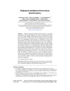
Figure 1. Schematic of a Michelson interferometer, where laser light is split into two arms by a beam splitter (BS), reflected by two mirrors (M1, M2), then recombined at the BS. A difference in arm length (∣ r1 − r2∣) results in a phase difference, ΔΦ , described by equation (5), and observed by the detector.
where (E10, E20 ) are the amplitudes and r1, r2 are the travel paths of each respective wave. 2π The wave vector, k , is a vector describing the propagation of the wave, where ∣ k ∣ = λ . The sum of these waves, E T , is given by
E T = E1 + E 2.
(2)
As we only detect the intensity of the resultant wave, at this point we convert from the electric field, E T , to the resultant intensity, IT:
IT = E 2T = ( E 1 + E 2 ) ∗ ( E 1 + E 2 ) = E 12 + E 22 + 2E 1 ∗ E 2 .
(3)
Given that
I1 = E 12
and
I2 = E 22 ,
(4)
the intensity of the summed plane waves of equation (1) is
IT = I1 + I2 + 2 I1 I2 cos (ΔΦ),
(5)
ΔΦ = k · r1 − k · r2 + ϕ − ϕ , = k · ( r1 − r2 ),
(6)
and
where r1 and r2 are the paths travelled by each wave and ΔΦ is the phase difference between the waves. For a Michelson interferometer, as shown in figure 1, the laser source is split into the reference and sample beams using a beam splitter, BS. Because the reference and sample beams have the same origin, there is no initial phase difference between the beams. The 3
Eur. J. Phys. 36 (2015) 035011
S Hitchman et al
beams are reflected by mirrors M1 and M2, and recombined at BS. The recombined beams are incident at the detector, the intensity of which is governed by equation (5). Equation (6) shows the phase difference at the detector is due to the optical path length difference between the two beams [9]. In a Michelson interferometer the reference mirror position is known (or constant) therefore the displacement of the sample mirror, M1, can be measured using the resultant intensity, IT. 2.1. The Doppler effect
From here on, we consider dynamic systems, where the the sample arm length r1 varies with time due to displacements x(t) of M1. In applications where particle displacements are small, but the angular frequency ω of the displacement is large, it stands to reason that the particle velocity v(t) is more easily detected [23]. Consider a sample with M1 in harmonic motion with an amplitude A:
x (t ) = A cos (ωt ).
(7)
Then, its particle velocity is defined by the temporal derivative:
v (t ) =
dx = ωA cos (ωt ). dt
(8)
This implies that for large values of ω, the particle velocity is relatively large compared to the particle displacement. In that case, we focus our detection scheme on the Doppler shift. In a Michelson interferometer, a stationary receiver detects light that is reflected off a moving target with particle velocity v(t). The detected frequency of the reflected light is Doppler shifted [7]. For a beam with normal incident to the surface of the mirror, that is, cos α = cos β = 1 in equation (8) of [7], and the detected signal has a frequency
⎛ 1 − v (t ) c ⎞ f2 (t ) = f1 ⎜ ⎟, ⎝ 1 + v (t ) c ⎠
(9)
where f1 is the emitted frequency, c is the speed of light and v(t) is the mirror velocity. For vs (t ) ≪ c , equation (9) can be further simplified using the Taylor series expansion
f2 (t ) = f1 (1 − v (t ) c)(1 + v (t ) c)−1 ≈ f1 (1 − v (t ) c)(1 − v (t ) c) ≈ f1 (1 − 2v (t ) c),
(10)
ignoring higher order terms. The Doppler shift is then given by
fD (t ) = f2 (t ) − f1 ≈ −
2v ( t ) , λ
(11)
where the wavelength of the source laser is λ = c f1. In interferometry only the motion parallel to the beam direction is considered; we define sample motion towards the beam as negative, resulting in positive Doppler shifts, and motion away from the beam as positive, resulting in negative Doppler shifts. As the reference and sample beams no longer have the same frequency, the intensity of the combined beams will ‘beat’ sinusoidally, with a frequency equal to the difference between the arms, caused by the Doppler shift. When beams of differing frequency superimpose, an additional amplitude modulation term arises in the interference term. This phenomenon occurs for all waves and is often referred to as ‘beating’. Again consider two plane waves, however this time with different frequencies and initial phase differences ignored: 4
Eur. J. Phys. 36 (2015) 035011
S Hitchman et al
(
)
E 1 = E10 cos 2πf1 t ,
(
)
E 2 = E 20 cos 2πf2 t ,
(12)
where f2 = f1 + fD . Converting to exponential notation, the superposition of these waves is given by
E T = E10 e i2πf1 t + E 20 e i2π ( f1 + fD ) t = e i2πf1 t ⎡⎣ E10 + E 20 e i2πfD t⎤⎦ .
(13)
Using the identity cos (2πft ) = Re [e i2πft], the resultant electric field is described a plane wave with a time-varying amplitude, defined by the term in the square brackets. Again we only detect the intensity of the resultant wave, which is given by
(
)
I = I1 + I2 + 2 I1 I2 cos 2πfD (t ) t .
(14)
2.2. Heterodyne interferometry
The intensity pattern described by equation (14) will produce the same beat pattern for positive and negative Doppler shifts of equal magnitude. Thus it can be said that the Michelson interferometer suffers from directional ambiguity. To turn this detector from a homodyne to a heterodyne device capable of extracting directional information of the particle velocity, a constant frequency shift can be added to the reference beam. The reference beam is then given by
( (
))
E 2 = E 20 cos 2π f1 + fC t . The beat frequency is therefore no longer only proportional to the magnitude of the Doppler shift, but the sum of the Doppler shift and the constant shift fC. This method removes several practical concerns. In particular the directional ambiguity due to the cosine function is removed, as a positive beat frequency is ensured, so long as fC is greater than fD. The information dependence on the magnitude of the intensity of each arm, I1 and I2, is also removed, as the information is encoded entirely in the oscillation frequency. Removing the DC terms, reducing the amplitude of the interference term to a single term and including the additional frequency shift, equation (14) becomes
( ( = A cos ( 2π ( f
)) C + hv (t ) ) t ) ,
Iac (t ) = A cos 2π fC + fD (t ) t
(15)
where A = 2 I1 I2 and h = 2 λ . IAC is analogous to a frequency modulated signal, where the message signal is the particle velocity of the sample, v(t), and h is the modulation index [8] which relates the observed frequency deviation to the message signal. As we are interested in the sample motion, frequency demodulation techniques used in communications can be applied to the intensity signal in order to extract the velocity information. In practice, fC is introduced with an acousto-optic modulator (AOM). AOMs use acoustic waves to produce gradients in the refractive index, n, of an optical medium. This occurs due to the dependence of the refractive index on the density of the medium, which changes with the acoustic wave. Although the changes in refractive index are relatively small (10−4), AOMs can have a large impact on the properties of the incident optical beam [12]. The refractive index gradient acts as a Bragg grating travelling through the medium with the acoustic wave. Unlike a stationary grating, each diffraction order also has a frequency shift of n ∗ fAOM , where n is the diffraction order and fAOM is the frequency of the acoustic wave. The frequency shift is typically in the Megahertz range, thus many orders of magnitude less than the oscillation 5
Eur. J. Phys. 36 (2015) 035011
S Hitchman et al
frequency of the incident beam. An excellent description of AOMs and Bragg gratings, including the governing mathematics, is presented in [33]. 2.3. FM Demodulation
As described by equation (15), the detected interferometer signal is frequency modulated, where the sample velocity is the message signal. Frequency modulation is a form of angle modulation, where the frequency of a carrier wave is modulated in accordance with some message signal. For a message signal of v(t), such as that in equation (15), the instantaneous frequency is
fi (t ) = fC + hv (t ).
(16)
Equation (11) shows h to be 2 for frequency deviations due entirely to Doppler shift, λ such as those in heterodyne interferometry. The detected interference pattern, IAC(t), must be demodulated to extract the particle velocity information. Demodulation can be performed digitally, but it requires high sampling rates (and thus large data sets per recording) to not alias the signal dominated by the carrier frequency. Performing analog demodulation removes these limitations. A phase locked loop (PLL) is a simple and effective electric circuit for frequency demodulation, provided high-quality radio frequency (RF) components are used [22]. A schematic of a standard PLL designed to demodulate a frequency modulated input signal is presented in figure 3. A PLL is a feedback system designed to adjust a voltage controlled oscillator (VCO) such that its oscillation frequency, flo(t), is matched to the input signal, IAC(t). Frequency matching is achieved by ‘locking’ the phase difference between the signals to a constant value. A frequency mixer and low-pass filter are often used as a differential phase detector, producing an output voltage, Vout, proportional to the phase difference between the input signals, rlo(t) and IAC(t). If there is a difference in frequency between rlo(t) and IAC(t), the phase difference between the signals will increase. The output of the phase detector follows this difference, and is used to control the frequency of rlo(t). The oscillation frequency of rlo(t) increases or decreases with the phase difference until the frequency matches the frequency of IAC(t). When the frequencies are matched, the phase difference between the signals is maintained. If the input signal is frequency modulated, the output of the PLL will ‘follow’ the frequency deviation, thus demodulating the message signal from the carrier. Typically VCOs require Vout to be offset by a DC voltage, VDC, in order to match the rlo frequency to the IAC carrier at Vout = 0 V. That is: flo ∝ VDC + Vout (t ). The low-pass filter determines several parameters of the PLL, particularly the maximum message frequency that can be demodulated and the noise floor. The PLL filter should be as close as possible to the maximum expected frequency, as a filter with high cut off frequency is not as effective at removing fC from the output signal. 3. The OSLDV: a simple LDV Figure 2 illustrates the design of the OSLDV. Light from a 1.2 mW stabilized helium–neon laser is split into the reference arm and sample arm with beam splitter BS1. The coherence length of this laser is such that it can accommodate a large optical path length difference between the reference and sample arms [33]. Due to the scattering and absorption losses of light from the sample, a greater interference amplitude is achieved by using a 90:10 (R:T) beam splitter (BS1); 90% of the beam energy is used for the sample beam and 10% is used for the reference beam. The sample beam is directed to the focusing elements through a polarizing beam splitter, PBS, which is orientated such that light from BS1 transmitted. Scattered 6
Eur. J. Phys. 36 (2015) 035011
S Hitchman et al
Figure 2. Schematic of OSLDV. M1-2: silver mirrors. AOM: acousto-optic modulator.
BS1: 90:10(R:T) beam splitter. BS2: 50:50 (R:T) beam splitter. PBS: polarizing beam splitter. Quarter and half wave plates are used to ensure that all light reflected from the sample is directed towards BS2, and to improve interference.
light returning from the sample has made a double pass through a quarter-wave plate, which rotates the polarization such that returning light is entirely reflected by PBS. Wave plates use birefringence to rotate the polarization of light; a half wave plate (or a double pass through a quarter wave plate) will rotate the polarization of light by 90° [9, 11]. The beams are recombined using a 50:50 non-polarizing beam splitter, BS2. BS2 produces two identical beams which both can be used in a single or double balanced detector configurations. For the 7
Eur. J. Phys. 36 (2015) 035011
S Hitchman et al
Figure 3. Schematic of the phase locked loop (PLL). VCO: voltage controlled
oscillator, LPF: low pass filter. Vout(t) is the output signal of the PLL which is proportional to the frequency deviation from the carrier, fD. A DC offset, VDC is applied to the VCO in order to match rlo(t) to the carrier frequency of IAC(t) at Vout (t ) = 0 . The amplifier has a gain of k = 24.4 to produce a sensitivity of 50 mm s−1 V−1.
Figure 4. Comparing velocity measurements of a vibrating plate at 100 Hz using the
OSLDV and a Polytec vibrometer.
OSLDV we use a single detector and terminate the other beam using a beam dump. An AOM in the reference arm increases the reference beam frequency by 80 MHz. The absolute value of the frequency shift is arbitrary, as long as it is significantly above the maximum expected Doppler shift caused by the sample motion. Thus the choice of AOM falls primarily to other properties, such as efficiency and aperture size. For the OSLDV a high diffraction efficiency (85%) fused silica AOM was used. Using the first order diffracted beam of the AOM as the reference beam, the output intensity ‘beats’ with frequency of 80 MHz for a stationary sample. When the sample is in motion the velocity is encoded in the frequency deviation from the carrier frequency due to the Doppler shift of the reflected light. Thus the interferometer
8
Eur. J. Phys. 36 (2015) 035011
S Hitchman et al
Table 1. Bill of materials.
System PLL
Summing amplifier
Component
Brand
Model number
VCO
Minicircuits
Mixer Operational amplifier Resistors Capacitors
Minicircuits LT
ZX95-200+ / ZX95-100+ ZX05-1L-S+ LT1259
— — Minicircuits
— — ZHL-6A-S+
Laser (HeNe) AOM
Thorlabs Gooch & Housego Gooch & Housego Thorlabs Thorlabs Thorlabs Thorlabs Thorlabs
HRS015 23080-1-LTD
RF amplifier Interferometer
AOM driver BS1 (90:10) BS2 (50:50) PBS Detector Mirrors (1–2)
21080-1AMXTL BS028 BS013 PBS102 FPD510-FV PF10-03-P01
produces a frequency modulated signal. Detection of this signal requires a detector that can resolve the high-frequency carrier signal, while still providing large gain. The OSLDV detector provides 4 ∗ 104 V W−1 for beat frequencies up to 250 MHz. Though not necessary, an electrical amplifier (ZHL-6A-S+) was used to amplify the detector output. This reduces the dependence of the demodulated signal on alignment of the focusing elements. All components for the OSLDV are mounted on a stiff aluminium plate with M6threaded holes, and are listed in table 1. The velocity sensitivity of the OSLDV demodulator can be calculated by dividing the sensitivity of the VCO used by the modulation index, h, 2 from equation (15) [22]. For h = λ ≃ 3.16 × 10⁶ Hz ms−1 and VCO tuning sensitivity of 3.87 MHz V−1 (Zx95-100-s+), the velocity sensitivity is calculated to be 1.22 ms−1 V−1. This is then amplified using a high-bandwidth current feedback oscillator to increase the sensitivity to 50 mm s−1 V−1.
4. Results To test the performance of the OSLDV we detect the particle velocity of a sinusoidal vibrating piston at low frequencies, as well as ultrasound waves in a mudstone sample, stimulated with a PZT. The detected waveforms are then compared to a state-of-the-art LDV system: the Polytec OFV-505 sensor head coupled with the OFV-5000 controller. Polytec OFV-505 systems have been used by many in research environments [15, 21, 29, 30], and allow for automatic beam focusing with large dynamic range and wide demodulating bandwidths.
9
Eur. J. Phys. 36 (2015) 035011
S Hitchman et al
Figure 5. Power spectra of 100 Hz vibrations using the OSLDV and Polytec vibrometers.
4.1. Low-Frequency oscillations of a piston
A Brüel & Kjær mini-shaker type 4810 driven with a frequency of 100 Hz was used to test the OSLDV at lower frequency, large displacement conditions. The measured velocity of the sample using the Polytec and OSLDV systems are presented in figure 4. Both the Polytec LDV and OSLDV waveforms are the average of 200 measurements, and acquired at 10 kilosamples per second with 16 bit resolution on an AlazarTech PCI oscilloscope card. The power spectra, presented in figure 5, show a small harmonic peak at 200 Hz in both traces, as well as greater noise in the OSLDV measurement. 4.2. Ultrasound in a mudstone
The anisotropic properties of mudstones have been extensively studied using PZT ultrasonic systems (e.g., [6, 10, 32]). We excite an ultrasonic wave with a central frequency of 500 kHz with an Olympus pulser (Olympus NDT 5077PR-20-A) and PZT (Olympus NDT V101RB) into a 37.5 mm diameter, 32.7 mm long, cylindrical core carbonate mudstone from the Bakken formation, with sedimentary layers perpendicular to the wave propagation. Measurements were recorded at room temperature and pressure. The compressional (P-)wave propagates through this mudstone at a speed of ∼3250 m s−1 [1]. For calibration purposes, we compare measurements of the particle velocity to the results of the Polytec OFV-505 sensor head, coupled with the OFV-5000 vibrometer controller with the VD-09 decoder. We use reflective tape on the mudstone sample to ensure enough light is reflected to the detectors of both LDVs. Acquisition was done using the 50 mm s−1 V−1 setting on the Polytec LDV, which is capable of detecting waves up to 1.5 MHz. Both the Polytec LDV and OSLDV waveforms are the average of 200 measurements, and acquired at 100 mega-samples per second with 14 bit resolution on an AlazarTech PCI oscilloscope card. The normalized cross correlation of the two recordings was calculated to be 0.97, at a time delay of 8.2 μs, which has been removed in figure 6 to visually assess the agreement between the detected waveforms The delay is introduced to the Polytec waveform due to the (proprietary) steps in its signal decoder. This delay is quoted in the Polytec manual 10
Eur. J. Phys. 36 (2015) 035011
S Hitchman et al
Figure 6. Ultrasonic wave field in a mudstone, measured with the Polytec and OSLDV vibrometers (after removing the documented delay in the Polytec measurement). The primary wave arrives at 10.5 μs, followed by waves scattered by the sides of the sample and internal heterogeneity.
Figure 7. Power spectra of the waveforms measured with the OSLDV and
Polytec LDV.
is 8.16 μs. With a sample thickness of 3.3 cm, the expected P-wave arrival time of 10.5 μs matches our observations. Later arrivals from a combination of reflections from the sides of the sample, scattering from internal heterogeneities, and ringing of the PZT source are recorded similarly on the two LDVs. The power spectra of the Polytec and OSLDV systems are presented in figure 7. The OSLDV has a higher noise floor at frequencies above 1.5 MHz, which is quoted to the maximum detectable frequency of the VD-09 decoder.
11
Eur. J. Phys. 36 (2015) 035011
S Hitchman et al
5. Conclusions With the development of many applications in non-contacting ultrasonics and acoustics, a low-cost OSLDV is presented as an alternative to commercial devices. Particle velocity encoding in the raw signals of an interferometer intensity signal is fully discussed, in addition to the extraction of the velocity information using electronic frequency demodulation techniques. The first acoustic and ultrasonic measurements of particle velocities in a mudstone and an aluminum plate prove virtually identical results, compared to a commercial system for frequencies from 100 to 1 MHz.
Acknowledgments Funding for this project was provided by The University of Auckland Faculty Research Development Fund. We thank the members of the Physical Acoustics Lab for their enthusiasm and support.
References [1] Adam L, Ou F, Strachan L, Johnson J, van Wijk K and Field B 2014 Mudstone P-wave anisotropy measurements with non-contacting lasers under confining pressure SEG Technical Program Expanded Abstracts [2] Argo T F IV, Wilson P S and Palan V 2008 Measurement of the resonance frequency of single bubbles using a laser doppler vibrometer J. Acoust. Soc. Am. 123 EL121–5 [3] Blum T E, van Wijk K, Pouet B and Wartelle A 2010 Multicomponent wavefield characterization with a novel scanning laser interferometer Rev. Sci. Instrum. 81 073101 [4] Castellini P, Martarelli M and Tomasini E 2006 Laser Doppler vibrometry: development of advanced solutions answering to technologyʼs needs Mech. Syst. Signal Process. 20 1265–85 [5] Castellini P and Scalise L 1999 Teeth mobility measurement by laser doppler vibrometer Rev. Sci. Instrum. 70 2850–5 [6] Dewhurst D N and Siggins A F 2006 Impact of fabric, microcracks and stress field on shale anisotropy Geophys. J. Int. 165 135–48 [7] Gjurchinovski A 2005 The Doppler effect from a uniformly moving mirror Eur. J. Phys. 26 643 [8] Haykin S 2009 Communication Systems (New York: Wiley) [9] Hecht E 2001 Optics 4th edn (Reading, MA: Addison-Wesley) [10] Hornby B E 1998 Experimental laboratory determination of the dynamic elastic properties of wet drained shales J. Geophys. Res. 103 945–64 [11] Hu Y, Yi Z, Yang H and Xiao J 2013 A simple method to measure the thickness and order number of a wave plate Eur. J. Phys. 34 1167 [12] Hunsperger R G 2009 Acousto-optic modulators Integrated Optics (Berlin: Springer) pp 201–20 [13] Johnson J L, van Wijk K and Sabick M 2014 Characterizing phantom arteries with multi-channel laser ultrasonics and photo-acoustics Ultrasound Med. Biol. 40 513–20 [14] Lauxmann M, Eiber A, Heckeler C, Ihrle S, Chatzimichalis M, Huber A and Sim J 2012 In-plane motions of the stapes in human ears J. Acoust. Soc. Am. 132 3280–91 [15] Lebedev M, Bóna A, Pevzner R and Gurevich B 2011 Elastic anisotropy estimation from laboratory measurements of velocity and polarization of quasi-P-waves using laser interferometry Geophysics 76 WA83–9 [16] Michelson A A 1881 The relative motion of the earth and of the luminiferous ether Am. J. Sci. 128 120–9 [17] Miffre A, Delhuille R, de Lesegno B V, Büchner M, Rizzo C and Vigué J 2002 The three-grating Mach–Zehnder optical interferometer: a tutorial approach using particle optics Eur. J. Phys. 23 623 [18] Nakamura K 2012 Ultrasonic Transducers: Materials and Design for Sensors Actuators and Medical Applications (Amsterdam: Elsevier) 12
Eur. J. Phys. 36 (2015) 035011
S Hitchman et al
[19] Ramamoorthy S K, Kane Y and Turner J A 2004 Ultrasound diffusion for crack depth determination in concrete J. Acoust. Soc. Am. 115 523–9 [20] Salman M and Sabra K G 2013 Surface wave measurements using a single continuously scanning laser doppler vibrometer: application to elastography J. Acoust. Soc. Am. 133 1245–54 [21] Scales J A and Malcolm A E 2003 Laser characterization of ultrasonic wave propagation in random media Phys. Rev. E 67 046618 [22] Schilt S, Bucalovic N, Tombez L, Dolgovskiy V, Schori C, Di Domenico G, Zaffalon M and Thomann P 2011 Frequency discriminators for the characterization of narrow-spectrum heterodyne beat signals: application to the measurement of a sub-hertz carrier-envelope-offset beat in an optical frequency comb Rev. Sci. Instrum. 82 123116 [23] Scruby C B and Drain L E 1990 Laser Ultrasonics: Techniques and Applications (Bristol: Hilger) [24] Sehgal C 1993 Quantitative relationship between tissue composition and scattering of ultrasound J. Acoust. Soc. Am. 94 1944–52 [25] Smith M L, Scales J A, Weiss M and Zadler B 2010 A low-cost millimeter wave interferometer for remote vibration sensing J. Appl. Phys. 108 024902 [26] Tramannoni F and Matteucci G 2006 Basic experiments of physical optics presented with a modified version of the Michelson interferometer Eur. J. Phys. 27 1267 [27] Turner J A and Weaver R L 1994 Radiative transfer of ultrasound J. Acoust. Soc. Am. 96 3654–74 [28] Valeau V, Sabatier J, Costley R D and Xiang N 2004 Development of a time-frequency representation for acoustic detection of buried objects J. Acoust. Soc. Am. 116 2984–95 [29] van Wijk K, Haney M and Scales J A 2004 1D energy transport in a strongly scattering laboratory model Phys. Rev. E 69 036611 [30] van Wijk K, Komatitsch D, Scales J A and Tromp J 2004 Analysis of strong scattering at the micro-scale J. Acoust. Soc. Am. 115 1006–11 [31] Vanlanduit S, Vanherzeele J, Guillaume P and de Sitter G 2005 Absorption measurement of acoustic materials using a scanning laser Doppler vibrometer J. Acoust. Soc. Am. 117 1168–72 [32] Wong R, Schmitt D, Collis D and Gautam R 2008 Inherent transversely isotropic elastic parameters of over-consolidated shale measured by ultrasonic waves and their comparison with static and acoustic in situ log measurements J. Geophys. Eng. 5 103 [33] Yariv A and Yeh P 2006 Photonics: Optical Electronics in Modern Communications (The Oxford Series in Electrical and Computer Engineering) (Oxford: Oxford University Press)
13