Heterogeneity as Key Feature of High Performance Computing: the ...

Heterogeneity as Key Feature of High Performance Computing: the PQE1 Prototype ♦ P.Palazzari1, L.Arcipiani1, M.Celino1, R. Guadagni2, A.Marongiu1, A.Mathis1, P.Novelli1, V.Rosato1 (1($ &DVDFFLD 5HVHDUFK &HQWHU ² 5RPH

+3&1

3URMHFW 

)XQ]LRQH

&HQWUDOH ,QIRUPDWLFD

SDOD]]DUL#FDVDFFLDHQHDLW

Abstract In this work we present the results of a project aimed at assembling an hybrid massively parallel machine, the PQE1 prototype, devoted to the simulation of complex physical models. The analysis of some of the existing parallel architectures has revealed that general-purpose machines are largely over-dimensioned and often perform inefficiently in grand-challenge scientific applications. We have thus developed an heterogeneous parallel system which matches task-heterogeneity with architecture-heterogeneity: in fact special-purpose massively parallel architectures, when coupled to general-purpose machines, are able to efficiently satisfy the requirements of complex scientific computing. We present the HW structure and the SW tools developed for the PQE1 prototype. Starting from the concept of machine-granularity and task-granularity, we show the necessity to exploit both high granularity and low granularity parallelism to efficiently use the PQE1 system. Some examples describing application fields in which the PQE1 prototype has been successfully used are briefly described.

1. Introduction Technical applications (image processing, real-time control,…) and simulation of complex models used in scientific applications (quantum chemistry, weather forecast, electromagnetic compatibility…) require sustained computational powers of the order of tens (or hundreds) of Gflops (1Gflops = 109 floating point operations per second). Massively parallel processing seems to be the only practical way to reach these figures. To date, commodity off-the-shelf processors are able to ♦

provide peak performance in the range of 1÷2 Gflops (for example, the 667 MHz Alpha 21264 chip has a peak performance of 1.3 Gflops [1]): hundreds of those processors can be coupled, for instance, up to reaching the desired sustained performances. The Accelerated Strategic Computing Initiative (ASCI, [2]) and the Path Forward project, finalized to build very powerful parallel machines to implement extremely complex simulations, have produced, to date, the installation of several general purpose platforms: 1. ASCI Red: composed by 9,216 Pentium Pro processors, has 584.5 Gbytes of RAM, bi-directional cross-section bandwidth of 51.6 Gbyte/sec and peak performance of 1.8 Tflops; 2. ASCI Blue Mountain: assembled with 48 Silicon Graphics/Cray Origin2000 servers (each is configured with 128 SMP processors) containing a total of 6,144 processors, with projected peak performance of 3 Tflops; 3. ASCI Blue Pacific: has 1,344 PowerPC 604e processors (332 MHz), 504 Gbytes of RAM, nodes connected through an Omega Network with a node-to-node bandwidth of 150MB/sec and offers a peak performance of 0.89 Tflops. Also these platforms, like the most widespread commercial parallel systems, are based on commercial general-purpose computing devices which allow to sustain very irregular programming models. If, on one side, this property makes these systems well suited for most of the computational tasks related to complex scientific applications, on the other side this can also be considered as their main limitation. In fact, the need of being general-purpose implies that these systems are designed to support multitasking/multiuser operative environments, so that most of their silicon, instead of

This work has been performed in the framework of an industrial collaboration between ENEA (The Italian Agency for New Technologies, Energy and the Environment) and QSW (Quadrics Supercomputing World Ltd., a Finmeccanica group company).

being devoted to implement computing devices, is used to build cache memory and control HW to manage complex memory hierarchies, out of order execution of instructions, processor scheduling and multiprocess environment. This fact, while enhancing system operability, largely decreases the efficiency per silicon area in floating point dominated applications, being a large part of the electronic devices not operative for most of the time [3]. A completely opposite approach to high performance scientific computing can be found in the physicists community, where small research groups are used to design by themselves dedicated machines which can efficiently solve their computational problems. An example of this approach is given by the GRAPE (GRAvitational PipE) system [4]: GRAPE-4, the system version now available, is a special purpose computer for astrophysical simulations (N-body gravitational problems requiring O(N2) computations) with peak speed exceeding 1 Tflops [5]. GRAPE system is a completely not programmable machine, allowing only to load/read initial/final data into/from the machine. Extreme specialization is the key to achieve very high efficiency in the use of the silicon area: in such platforms only the required functions are implemented, thus maximizing the performances per unit of volume of electronics. The GRAPE project is going to release a 200 TFlops computer [6], yielding a computational speed from 10 to 100 times larger than that achievable, on the same problem, in the platforms developed in the framework of ASCI project. A further example of the advantages which can be achieved through HW specialization is given by the APE project [7] launched by Italian physicists, aimed to build a massively parallel system to be used in Lattice Quantum Chromo Dynamics (LQCD). These platforms, the APE series (APE100 is the old system [8], APEmille is the new prototype which will be soon launched [9],[10]) are SIMD programmable systems equipped with up to 2048 Very Long Instruction Word (VLIW) custom processors and offering peak performances of 100Gflops (APE100 series) and 1 Tflops (the new APEmille system). In both cases, the machines in the largest configurations are easily contained in few rack-mounted containers. In scientific computations, most of the time is usually spent in the execution of quite regular codes which iterate (e.g. in time, frequency, space) several transformations on large domains of data. In such a computational scenario, heterogeneous computing is a very promising way to achieve high performances: the key idea is to connect a (small) general-purpose parallel machine to several, very powerful, specialized parallel systems. The less flexible, specialized machines are dedicated to provide most of the computational power required by the numerical programs, while the general-purpose machine is used to give the necessary flexibility to the whole system, coordinating

tasks and pre/post processing data produced by the specialized systems. Heterogeneous computing has been used to achieve the very high performances required when dealing with challenging problems: machine heterogeneity is exploited to match task heterogeneity, using massively parallel systems as dedicated, high-efficiency boosters attached to a single user general-purpose parallel machine. In this work we present the outcome of a scientific program aimed at developing a massively parallel hybrid machine. In the first part of the paper a theoretical framework to describe heterogeneous tasks and heterogeneous systems is presented. Task and machine granularity are introduced and their influence on the efficient implementation of heterogeneous tasks onto heterogeneous systems is discussed. Then we describe the PQE1 prototype, the massively parallel hybrid system which has been developed in our research center. Along with the description of the HW and the SW of the system, we discuss the rationale of such architecture and we sketch the results obtained in two different, successful applications of the PQE1 platform. Finally the next version of this hybrid prototype, now in its final design phase, is presented.

2. Hierarchical Modeling of Heterogeneous Tasks and Systems An algorithm to be implemented on a parallel system can be represented as a labeled Control Data Flow Graph (CDFG) G(N,E,C_N,C_E), being 1. N={ni | i=1,2,…,N} the set of functionality necessary to implement the algorithm, 2. E⊆N×N={eij=(ni,nj)| ni sends data to nj} the internode communication set, 3. C_N={c_ni | c_ni ∈ℵ, ni ∈N, i=1,2,…,N} the node labeling set, containing the integer value which is a measure of the complexity of the functionality corresponding to ni (e.g., the number of operations needed to implement ni) and 4. C_E={c_eij | c_eij ∈ℵ, eij ∈E} the channel labeling set, containing the integer value which is a measure of the complexity of the communication corresponding to eij (e.g., the number Data_in1 … Data_inN_ini ek1i … ek i N_ini ni,c_ni

⇔

eik1 … eikN_out

fi(Data_in1,…,Data_inN_in_i, Data_out1,…,Data_outN_out_i)

i

Data_out1 … Data_outN_ini Figure 1: graph node, with input and output edges, representing the computation ni.

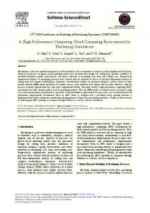
modeled through another task or parallel system graph: such a hierarchical description of a graph allows to put in evidence only the degree of parallelism (and of detail) which the user wants to consider. All the lower level details are hidden at this stage of abstraction. For instance, a complex program can be represented through a CDFG in which nodes are very complex routines; after a refinement step, each routine can be detailed through several simpler routines (for instance, an iterative solver can be expressed by means of Basic Linear Algebra Subroutines (BLAS)); going on with the zooming of details, each BLAS routine can be decomposed into (dependent, i.e. interconnected) elementary operations expressed in a standard imperative language (e.g., C or Fortran). As example of hierarchical representation of a parallel system, we can think to a system graph whose nodes are large systems (Vector Computers, Distributed Memory SIMD and MIMD systems, Shared Memory Multiprocessors, DSP and specialized computing devices) connected through some kind of (eventually not homogeneous) IN. Each node can be detailed through several lower level nodes (processors of the system and their IN) which can still be detailed through a lower level representation (interconnected functional units within a processor). A sketch of this hierarchical description is SIMD PE PE PE CU

SIMD SIMD MIMD

PE PE PE PE PE PE

MIMD Vector Proc

Figure 2: Hierarchical representation of a heterogeneous parallel system

Data DRAM

of byte sent through eij). Each node ni in the computation is associated to a functionality which transforms N_ini input data (with their corresponding associated data type) into N_outi output data (with their data type). N_ini and N_outi are, respectively, the input and the output degrees of ni. The correspondence between node ni and function fi is depicted in figure 1. In a completely similar way, a parallel system can be represented through a labeled graph PS(R,IN,M_R,B_IN), being 1. R={ri | i=1,2,…,r} the resource set (processing elements with their local memory, shared memory banks, I/O devices) which can be decomposed into basic sets, i.e. R={∪i=1,..,kpi}∪{∪i=1,..,mMi }∪{∪i=1,..,tI/0i }. So the parallel system resource set is constituted by - k sets of processing elements pi, each set pi being characterized by the number and by the type of homogeneous computing devices contained in it; - m sets of memory banks Mi, each set of memory banks being characterized by the number of memory banks, by their access time and by the size of each bank given (in byte) by sizeof(mj), mj∈Mi; - t sets of I/O channels I/Oi, each set being characterized by the directionality, the bandwidth and the number of channels contained in it. 2. IN⊆Pow(R)×Pow(R)={cij=({ri1,…,rih},{rj1,…,rjn})| {ri1,…,rih} is connected to {rj1,…,rjn}} the interconnection network set, where Pow(R) denotes the power set of R. Pow(R) is used to model shared interconnections: a set of homogeneous processors pi={p,p,…,p} sharing a memory bank m∈Mi are represented through the couple (pi,m); a shared bus connecting the processors of pi is represented by the couple (pi,pi); a point to point connection with one dedicated channel between two not homogeneous processors is represented by the couple (pa∈pi, pb∈pj); 3. M_R={m_ri | m_ri ∈ℵ ri ∈R, i=1,2,…,r} the resource labeling set, which associates to each resource a number measuring its performances (e.g. the number of flops executed per clock cycle by a general purpose processor p∈pi, the number of clock cycles necessary to compute functionality f in the computing devices dedicated to its HW implementation, the access time for shared memory banks m∈Mi, the bandwidth for I/O channels c_i/o∈I/Oi); 4. B_IN={b_cij | b_cij ∈ℵ, cij ∈IN} the labeling set which associates the bandwidth to each channel cij∈IN. It is fundamental to underline that, in the cases of both task and parallel system graphs, each node can be

FU1 FU2

FUn

Register File

depicted in the example reported in figure 2.

3. Task and Machine Granularity: Formal Definition of Heterogeneous Systems and Heterogeneous Tasks Once introduced the formal hierarchical definitions to model computations and parallel systems, we try to give a (not exhaustive) definition of task and system heterogeneity. We need first to introduce the fundamental concepts of task and machine granularity.

The granularity of a task is usually referred to as being proportional to the ratio between the computation and the communication times involved in the execution of the task [23]. This definition of granularity is, indeed, machine dependent, as both communication and computation times may vary when the task is executed on different architectures. Being interested to a heterogeneous environment, we prefer to introduce the concepts of machine granularity (gm) and task granularity (gt). gm is a measure of the balance between computational and communication speed of a system and is defined as gm =

node peak computation speed PCS = (1) I/O bandwidth BW

where the node peak computation speed (PCS) is the maximal number of operations per second executed by the node (usually PCS are expressed in terms of flops in the context of numerical computations). Previous definition can be applied to nodes at different hierarchical levels. Referring to figure 2, for instance, we can define the granularity of vector nodes, SIMD nodes and MIMD nodes; at this level (the system level) nodes usually have very high granularity gm, ranging typical computation speeds from few Gflops to several tens of Gflops and typical I/O bandwidth from tens of Mbyte/sec up to few Gbyte/sec (for massively system with parallel fast I/O); a typical value for a medium-large system can be gm =

50 × 10 9

= 100 . When moving to a lower level of

500 × 10 6 detail (the sub-system level), granularity of a node diminishes, as typical computation speeds of today’s processing elements are in the range of few hundreds of Mflops up to 1-2 Gflops and communication bandwidths range from tens up to few hundreds of Mbyte/sec; typical value for a high-end processing element (like the Alpha EV6.7) equipped with a 64-bit PCI connection is gm =

1.3 × 10 9

= 6.5 . Moving into a lower level of 200 × 10 6 detail (the processor level, inside the processing element), granularity assumes a smaller value, as communication speed is always in the range of few hundreds of Mflops up to few Gflops, while communication bandwidth (processor⇔memory) ranges from few hundreds of Mbyte/sec up to few Gbyte/sec; for instance, a processing element with an EV6.7 processor (peak speed 1.3 Gflops) and a fast chipset for the memory control (e.g the Tsunami chipset, allowing an internal memory bandwidth of 2.6Gbyte/sec) is characterized by a granularity gm =

1.3 × 10 9

= 0.5 . 2.6 × 10 9 We are now able to give the following definition of heterogeneous system: a parallel system is heterogeneous when

1. 2.

3.

it is composed by more than one computing element and its computing elements are based on different architectural paradigms (Vector systems, Distributed Memory/Shared Memory MIMD systems, SIMD systems, etc..) and/or it can be described through a hierarchical classification evidencing different node granularities throughout the hierarchical levels.

gm is a measure of the ratio between system computation speed and system communication bandwidth. Following a similar reasoning, task granularity gt is defined as a measure of the balancing of computational and communication requirements of a task and is defined as gt =

number of computing op. n_op = (2) number of bytes of I/O data n_I/O_byte

The hierarchical classification approach, used to model heterogeneous tasks, can be applied also in the case of CDFGs. Given a CDFG with k different nodes, gt(ni) is the granularity of each node (i=1,2,..,k; ni∈N) and the granularity of the whole CDFG is the maximal value of the granularity of its composing tasks, i.e. gt(CDFG)=maxi=1,k(gt(ni)) (3) Granularity of a set of nodes is defined as the largest granularity in the set because it seems to be reasonable to represent computation/communication demands of a complex task through its largest component; in fact, given for instance a CDFG with 9 different nodes with the same (small) granularity 1 and one node with (large) granularity 100, computation/communication demands are well represented by the value 100 (worst case). If we use an average value to represent the global task granularity, in previous example we would obtain gt=10.9, which clearly underestimates the influence of the ‘large’ task, probably yielding, as we will discuss later, an inefficient implementation of the task on the parallel system. When a hierarchical representation of a CDFG is used, the change from the procedural level (i.e. the level in which nodes represent routines) to the instruction level of detail (nodes represent elementary instruction, e.g. basic C statements) determines a decrease in the node granularity. In fact, if we indicate with n the size (in byte) of the input/output parameters, the number of operations N_OP(n) executed by the routine has, in most cases, a dependency law larger than O(n), i.e. N_OP(n)≥O(n). N_OP(n)=O(n) is a lower bound, being O(n) the number of elementary operations necessary to read/write input data (with the obvious exception of data structures already stored in memory and communicated through a pointer; however, also in this case the following inequality (4) is satisfied). As a consequence, the law connecting the

granularity of a task to the size n of input/output data is given by g t (n) =

N_OP(n) ≥ O(1) O(n)

(4)

At the instruction level the granularity is O(1), i.e. the number of bytes used to encode input and output parameters of one operation is a constant number (with very few, and particular, exceptions involving data movement), because elementary operations manipulate one or two scalar values and return another scalar value. As a consequence, when moving from the procedural to the instruction level, task granularity does not increase (typically diminishes). Other parameters characterizing nodes of CDFG, at the procedural level, are - the type T∈{‘control-dominated’, ‘computationdominated’}; a node is control dominated when has small granularity and contains a number of decision operations (i.e. conditional jumps) significantly larger than the computing operations; on the contrary, a node is computation dominated when has large granularity, - computational paradigm; each node of the graph, when expressed at a lower level of detail, can be represented by means of the ‘data-parallel’, the ‘pipeline’, the ‘farm’, the ‘loop’, the ‘unrestricted’ structuring constructs; for the description of the structuring constructs, except the ‘unrestricted’, see [29]; the ‘unrestricted’ paradigm refers to a generic computation represented by means of an irregular CDFG. We are now able to give the following definition of heterogeneous task: a CDFG represents an heterogeneous task when 1. it is composed by more than one node at the ‘procedural’ level and 2. its nodes are based on different computational paradigms or have different types T and/or 3. its nodes have different granularities

4. Matching Task and System Heterogeneity to Maximize System Performances Once fixed the meaning of heterogeneity for tasks and systems, it is important to evaluate their mutual relation and to describe the associated heterogeneity parameters (granularity, computational/architectural paradigms, node type T). In this framework, it is worth investigating the connections among system/task granularity, heterogeneity and global performances. The granularity G, in its classical form, is defined as the ratio between Run time (R) and Communication time (C) of a given task [28], i.e.

G=

task execution time R (5) = task communication time C

In order to avoid a too formal explanation, far beyond the scope of this paper, we do not go into the details necessary to define task execution and communication times; intuitively, we consider as execution (communication) time the summation of all the time intervals in which at least one computational unit (I/O channel) is computing (communicating). Previous definition of granularity is machine dependent, being execution and communication times connected to processor speeds and I/O bandwidths. The previously introduced definitions of gm and gt can be used to make explicit this dependence; in fact G can be expressed as G =η being η =

gt gm

(6)

η proc

an efficiency figure which takes into η comm account the partial utilization of the processor speed η proc and of the bandwidth (η comm ) . In order to verify

(

)

the validity of (6), it is sufficient to substitute in it the expressions of gt and gm and, with few algebraic operations, we obtain n_op η proc η proc g t n_I/0 _byte = = G= PCS η comm g m η comm BW n_op 1 R = η proc = n_I/O_byte C PCS η comm BW The actual value of η depends on the characteristics of tasks and on their implementation on the physical system. A reasonable estimation, to be confirmed through some experiences on a given system, is η=0.1÷0.5. For instance, when dealing with tasks with large I/O packets (small granularity), usually communication startup time is negligible and ηcomm≅1; in such a case η=ηproc and processor utilization in the range from 20% up to 60% is a realistic figure. The expression of G as ratio between task and machine granularity underlines how the relative values of task and machine granularity are relevant to achieve high performances when implementing the task on an actual (heterogeneous) parallel system. Efficient task implementation requires to match two conflicting behaviors: that of a task with maximum parallelism (to minimize execution time) with the constraint of minimizing communication costs (overheads). The only information on the granularity G is not sufficient to determine if the implementation of the task on a machine

is efficient: G gives just a measure of the relative influence of communication overhead on system performances. Given an implementation of a task on a parallel system, efficiency reaches its maximum when, for a fixed degree of parallelism, communication overhead is minimum. In fact, indicating with R the time spent executing computations and with C the time spent in communications, and defining as efficiency the ratio Eff =

R (7) Actual Computing Time

where the Actual Computing Time is the elapsed time from the start of the parallel program till its end, the following inequalities hold: R R ≤ Eff ≤ = Eff Max (8) R +C MAX(R, C)

Eff Min =

which can be rewritten, introducing the granularity G, as Eff Min =

1 1+

1 G

≤ Eff ≤

1 ) G

= Eff Max (9)

It is worthwhile to note that the fraction of unused computational resources is given by (1-Eff). The lowest value for the efficiency (EffMin) corresponds to the complete absence of overlapping between computation and communications; the highest value for the efficiency (EffMax) corresponds to a complete overlapping between computations and communications. In figure 3 the values EffMin anf EffMax are sketched as function of the granularity G. 1.2

Efficiency

1 0.8 0.6

Min Eff Max Eff

0.4 0.2 0 0

1

2

3

G>

Eff T 1 − Eff T

(10)

and, evidencing dependence of G on gt and gm, we obtain gt Eff T 1 > ⋅ g m 1 − Eff T η

(11)

Eff T 1 − Eff T we obtain a fundamental relation between task machine granularity: From previous inequality, setting

1 MAX(1,

negligible is the communication time with respect to computing time. Values of GEffT,

4 5 6 Granularity

7

8

9

10

Figure 3: Minimum and maximum efficiency values vs Granularity Actual efficiency values lie within the two plots, being closer to the lower or to the higher depending on the algorithm structure and the HW support for computation and communication overlapping (number of DMA channels, routing processors). G=1 indicates equality between computation and communication times. The larger is G, the more

k=

1 , η and

⋅

g t > k ⋅ g m (12) In the case of perfect overlapping between computation and communications, it is easy to verify that expression (12), from the position G>1, becomes gt >

1 ⋅ gm η

(13)

Previous expressions ensure a correct implementation of tasks on heterogeneous systems. The value k has to be estimated on the basis of ‘reasonable’ assumptions about the degree of overlapping between computations and communications (expression of k has been determined assuming the worst case, with no overlapping) and about the efficiency η which can be achieved when implementing the task on the system. The scheme to allocate a heterogeneous task onto a heterogeneous system is the following: - Consider the highest levels of detail both for the system and the task graphs; - Ordinate the node tasks in descending order of computational complexity; - For each node in the task graph, chosen according to previous decreasing ordering, select the system nodes which match, with their architectural paradigms, the node computational paradigm; - Among all the candidate system nodes, choose the one which has the highest computational power and respects the relation gt>k⋅gm; as the choice of the system depends on k, i.e. on the efficiency of the implementation of the task node on the system node, the process can be iterated at a lower level of detail

(i.e. the node is expanded (if possible) into a smaller granularity CDFG and also the system node is considered at a lower level of detail) until a reasonable estimation for k is achieved. - Assign the task node to the system node found in previous point (the choice of the system with the highest computational power allows to satisfy the tasks with highest computing requirements). As the previous ‘recipe’ does not consider the load balancing, some policy must be chosen to avoid the overloading of the most powerful systems; a method could be based on a cyclic allocation policy or on some dynamic updating of system performances (as a system node becomes more loaded, its computational speed appear smaller to the other task nodes that must still be allocated). In order to take into account precedence relations among nodes in the CDFG, techniques discussed in [23], [35] can be used.

5. The Heterogeneous PQE1 System The previous discussion is aimed at stressing that a heterogeneous system is not a mere collection of several platforms used, sometimes, as a parallel system, but it is an integrated system that must be designed from scratch to behave as a heterogeneous parallel system. In fact, heterogeneity is a property of the problems to be solved. A ‘well balanced’ heterogeneous system will thus provide the best way to solve complex ‘real’ problems. Heterogeneity moreover, avoids to over-dimension a parallel system, as the computational power is ‘dedicated’ (according to several computational paradigms), allowing very high efficiency. The idea is to avoid, as much as possible, the use of general purpose systems just because they perform ‘quite well’ in all the problems but not ‘very well’ for any problem. On the contrary, heterogeneous systems could contain different ‘dedicated’ parallel systems, some of which very well suited for a certain class of problems, others for others different classes. In this way, in principle, it would be possible to have a system which often behaves ‘very well’ on a lot of problems, because different parts of a complex application could be efficiently implemented onto architecturally different parts of the system. Furthermore, on the basis of the previous analysis, specialized architectures are, often, less costly (in terms of silicon area, power consumption, volume) than general purpose systems.

5.1

Rationale for the PQE1 prototype

General-purpose parallel machines support the Single Program Multiple Data (SPMD) asynchronous programming paradigm. Their HW structure is inherently asynchronous and some silicon area, other than some

time, must be wasted to manage process synchronization and asynchronous communications. Such a wasting of resources can be avoided by using synchronous machines to which could be efficiently allotted computational tasks requiring synchronous algorithms. On the basis of the experience gained using SIMD systems in several fields of technical-scientific computing (material science [14][15], astrophysics [40], atmospheric modeling [16], image processing and compression [17][18], computational electromagnetic [19][20], linear algebra [21], neural networks [22]) we are convinced that SIMD architectural paradigm can efficiently express programs solving problems related to such fields. Moreover it is also preferable to the MIMD paradigm because many algorithms 1. are synchronous; 2. often require that all the processors execute the same instructions on different domains; 3. need interprocessor communications executed in a synchronous way; 4. do not need deep memory hierarchies thanks to the regular patterns of memory accesses. Point 1 and 3 show that, for such classes of algorithms, the time spent in synchronization phases, required by MIMD systems, is a completely unnecessary overhead introduced by the asynchronous HW structure of the machine. This overhead is not required by SIMD machines with synchronous communications. Point 2 shows that all the HW dedicated to manage different program flows in the processors is unnecessary, being sufficient one centralized controller of program flow. Point 4 means that cache memory and the related management policies are not needed in most scientific applications, being the ‘locality’ of the problem [30] easily controlled by the programmer through instructions of vector movements between main memory and an internal register file. Although cache memory results to be particularly useful in multi-programmed environments, where several processes are running and the fast memory is not large enough to keep the whole image of all the running processes, in most cases of scientific computing only one process is running and its locality is easily captured by the programmer through instructions which allow burst memory transfers, through DMA channels, between the slow external RAM and a fast internal register file (or a multi-port/multi-bank internal static memory). A further discussion on SIMD vs MIMD architectures, along with a description of SIMD/MIMD mixed mode systems, is reported in [27].

5.2

HW description of the PQE1 prototype

The PQE1 is an ‘hybrid’ MIMD-SIMD platform where the flexibility and operability of a MIMD (distributed memory) architecture (the eight node Meiko/QSW CS-2) are coupled to the power and efficiency of SIMD

machines (7 APE100/Quadrics systems) which enable to efficiently perform in small granularity tasks. If we take into account the 4 points listed above and we assume that most algorithms arising in scientific applications can be expressed through synchronous programs with synchronous communications, executing the same instruction on a set of different data which can be easily mapped onto a data parallel structure with regular patterns of memory access, it results very reasonable to allot those parts of the computation to the SIMD machine APE100/Quadrics, leaving the remaining tasks of the computation to be executed on the MIMD part. We used 7 APE100/Quadrics machines, built in 1994: two with 512 processors arranged as an (8x8x8) 3D torus and 5 with 128 processors arranged as an (8x4x4) 3D torus. Each computing node is based on a custom VLIW processor, has clock frequency fck=25 MHz and is able to terminate a ‘normal operation’ A×B+C every clock cycle, so each processor executes two floating point operations in one clock cycle (when the pipeline is full) and has a peak speed of 50 Mflops; floating point are represented according to the IEEE 754 standard (single precision). Each node is connected to a data memory of 4Mbytes and has an internal register file (RF) with 128 registers; each clock cycle the processor is able to read two operands from RF and write one result to RF. Communications with other adjacent nodes, connected in the north, south, east, west, up and down directions are synchronous and memory mapped; interprocessor communication bandwidth is 12.5 Mbyte/sec, so the 512 (128) processor configuration has an aggregate bandwidth of 6.4 (1.6) Gbyte/sec and a peak speed of 25.6 (6.4) Gflops. The connection of the APE100/Quadrics machines to a MIMD system, the Meiko/QSW CS-2 [24], has been performed to give more flexibility to the SIMD machines. Each node of the MIMD platform is based on two Ultra Sparc processors, connected in the SMP configuration, it offers a peak speed of 180 Mflops and has 128 Mbytes of RAM. The connection between CS-2 nodes and APE100/Quadrics systems is implemented through an HiPPI (High Performance Parallel Interface) channel, which provides a bandwidth of 20 Mbyte/sec. The connection among the nodes of the CS-2 machine takes place via the Meiko/QSW proprietary network based on the ASIC circuits Elan/Elite and implementing a multistage interconnection network with Fat Tree topology and point-to-point bandwidth of 100 Mbyte/sec. The scheme of the complete prototype is shown in Fig.4. The PQE1 hybrid systems is thus composed by 7 SIMD machines which allow to obtain an aggregate computational speed of 83.2 Gflops, 20.8 Gbyte/sec of bandwidth and 6.5 Gbytes of RAM. These parallel systems communicate through 7 HiPPI channels with a CS-2 machines, so the communication bandwidth

between the two systems is 140 Mbytes/sec. The CS-2 MIMD parallel system has 8 twin nodes, offers a peak speed of 1Gflops, has 1 Gbyte of RAM and has an aggregate bandwidth of 800 Mbyte/sec. Looking at previous data, it is clear that the machine is strongly unbalanced, having the most of computational and communication speed in the SIMD part. If we analyze the sub-unit composed by a CS-2 node and the attached SIMD machine, seen as co-processing system, the

Node #0

APE 100

APE 100

APE 100

APE 100

APE 100

APE 100

APE 100

#512

#512

#128

#128

#128

#128

#128

Node #1

Node #2

Node #3

Node #4

Node #5

Node #6

Node #7

CS-2 Interconnection Network

Communication Interface Ultra Sparc

Ultra Sparc

Figure 4: HW structure of the PQE1 Prototype

128 Mbyte DRAM

resulting sub-unit granularity (at the system level) is g m ( APE100−#512) =

25.6 ⋅ 10 9 20 ⋅ 10 6

= 1280 (14)

and g m ( APE100−#128) = 320 (15) The PQE1 system can be considered, at a first level, as a parallel machine with small parallelism (parallelism degree is 7). In order to avoid wasting of performances, at this level of parallelization we have to consider only very large granularity tasks. If we consider, for instance, the product of two (n x n) single precision matrices, the task 2n 3

n (2n3 is the 6 12n number of operations required, while 12n2 is the number of byte to transfer, being necessary reading the two input matrices and writing the result matrix). In order to avoid I/O bound behavior, ηgt>gm must result; in the case of a 128 processor machine, supposing η=0.5 (reasonable value for this type of computations, using sequences of not independent operations of the type A×B+C), this corresponds to the condition n>3840. granularity is given by g t =

2

=

The second level of parallelism can be exploited within the single task. The SIMD machine has granularity (at the sub-system level) is gm =

25.6 6.4 = = 4 (16) 6.4 1.6

In this case we have a lot of parallelism available (parallelism degree is 128 or 512) and we can deal with small granularity tasks. As stated above, the rationale for such a strong machine imbalance is that SIMD systems are very well suited to implement numerical computations, allowing to reach very high sustained performances. The MIMD nodes are not devoted to solve the ‘number crunching’ part of the problem, but to perform data pre/post processing and to allow communications among different algorithms implemented on the SIMD systems. We underline that typical sustained performances obtained on the APE100/Quadrics machines range from 30% to 70% of the peak performances, i.e. they vary from 7.7 to 18 Gflops on the 512 node machines.

5.3 SW description of the PQE1 prototype The basic modality to program PQE1 system is the using of a message passing paradigm (the MPI library) to manage the high granularity tasks allocated into the MIMD part. In order to allow a low-level interaction between CS-2 nodes and SIMD machines, a communication library has been devised and implemented. This library contains a set of commands to load/run programs into the SIMD machines, to synchronize the execution between the program running on the MIMD node and the program running on the connected SIMD system, to communicate data to/from the SIMD system. Due to the large granularity of the programs running on the SIMD nodes, no particular effort has been spent to reduce start-up times which, for all the operations, are in the order of 10 ms. As the MIMD system is devoted to manage the whole hybrid system and to increase the flexibility of the PQE1 platform, a library implementing the functionality of a Distributed Virtual Shared Memory (DVSM) was developed [25]. This library allows to declare physically distributed memory areas as ‘shared’, thus allowing the user to operate on such areas with the usual operations of locking/unlocking and implementing atomic instructions to perform blocking/non-blocking read/write operations with synchronized/unsynchronized access. Typical times for locking (unlocking) an area are 60 (45) µs; the time necessary to access in writing (reading) a page is 19 (50) µs. Previous times do not depend on the size of the memory area. A further tool, called SkIE-CL [26], has been devised and implemented to improve the programmability of

PQE1 system, is a skeleton based coordination language which allows to express task/data parallelism through some predefined schemes (pipeline, farm, map, loop). Once the program has been written through the available parallel constructs, SkIE-CL is able to generate MPI code to program the MIMD part of the machine, performing a (near)-optimal mapping of tasks on the MIMD part of the system, by using some analytical model of the constructs; furthermore SkIE-CL allows to control the SIMD systems by means of the communication library described above. Previous tools (the DVSM and the SkIE-CL) were jointly developed by QSW and the Information Science Department of University of Pisa. Two interesting applications using PQE1 prototype features, i.e. overlapping computations between the SIMD and the MIMD parts of the system can be found in [21] and [16]. The first refers to the implementation of Basic Linear Algebra Subroutines-3 on the SIMD part of the system. The MIMD connections are used to perform a block-based partitioned matrix-matrix product, being the sub-blocks products distributed among several SIMD machines. The second work is related to the implementation of a high resolution meteorological limited area model coupled with an ocean model for the prediction of the state of the Mediterranean Sea and of high water events in the Venice Lagoon. The code was parallelized by allotting the computation of the most time consuming models (the High Resolution and the Very High Resolution Limited Area Models) to the SIMD part and the resolution of the less intensive computing spectral wave model (WAM) to the MIMD nodes. To these nodes is also demanded the computation of the two dimensional model (POM) for the prevision of the Adriatic Sea circulation and, ultimately, the finite elements shallow water model of the Venice Lagoon. In the following two paragraphs we give some details on the implementations and the results achieved when using the PQE1 system to perform n-body gravitational computations and electromagnetic simulations.

5.4 n-body computations The PQE1 architecture has been recently used for performing n-body (O(N2) calculations to study the dynamic behavior of a galactic globular cluster hosting a massive object (black hole) in its center [40]. Calculations have been carried out by exploiting a double level of parallelism which can be attained with the machine: the first, related to the SIMD parallelization of the O(N2) loop, was obtained by partitioning the stellar positions among the different nodes and by allotting the force calculations on the given partition to the single SIMD node. The hypersystolic loop ([36],[37)] has been successfully used to reduce communication times within the force loop calculation. The second level of parallelism has been exploited by using the MIMD resources to

evaluate the black hole-stars interactions (O(N) loop) during the time spent by the SIMD part to evaluate the interstellar interactions. The concurrent use of both the MIMD and the SIMD parts allowed to perform the integration of one reference time (crossing time) of a system of N=128000 stars in a CPU time of the order of t=72500 sec (with the SIMD part constituted by a platform with 512 nodes).

5.5 Electromagnetic simulation We investigated the simulation of dynamic evolution of electromagnetic fields through the integration of Maxwell equations by means of the Finite Difference in the Time Domain (FDTD) scheme. A domain with (n × n × n) cells was considered. Simulating one period of the input signal requires Ns time steps. At the end of each period of the simulation (i.e. at simulation time n+Ns, n=0,1,…) in each cell the value E max (i, j, k) =

( t =1,..., N max

s

E i,n +j, kt

)

is computed. These maximal values are then sub-sampled with step s and communicated to the host to be post-processed (for example reordered, normalized and stored). In order to simulate an EM phenomenon with frequency f=1.9 GHz on a domain with (n × n × n) cells, we have chosen spatial discretization ∆=1.5 cm and temporal discretization ∆t=2.88×10-11 [sec] to avoid numerical and modal dispersion, so Ns=19. The number of computations executed in one period is Nflops = Ns×36×n3=684n3 (17) Setting the sub-sampling step s=5 (i.e. two samples for wavelength are saved), at the end of each period the number of bytes to be sent is given by 3

4 3 n Nbytes = 4 ×   = n (18) s 125   According to (2), task granularity is given by 684n 3 = 21675 (19) 4 3 n 125 From (6), (14) and (19), assuming an efficiency in the implementation η=0.2, we obtain the granularity value for the EM simulation executed on the 512 processor APE100 system η ⋅ g t 0.2 × 21675 = ≅ 3.4 G(APE-#512) = gm 1280 and, from (6), (15) and (19) the granularity value for the execution on the 128 processor APE100 system η ⋅ g t 0.2 × 21675 = ≅ 13.5 G(APE-#128) = gm 320 gt =

Resulting G>1 in both previous cases, the simulation of one period of the EM phenomenon and the communication of sub-sampled results does not originate an I/O bound problem. The second level of parallelism can be exploited within the single FDTD task. In this case we have a lot of parallelism available (parallelism degree is 128 or 512) and we can deal with small granularity tasks. For example, going inside the structure of the parallel FDTD simulation (described in [20]), 36(nc)3 is the number of floating point operations executed in one time step within a processor where (nc × nc × nc) cells have been allocated and 2×6×4(nc)2 is the number of bytes to communicate at each time step (3 faces with two of the Ex, Ey, Ez components (depending on the face) and 3 faces with two of the Hx, Hy, Hz, components must be communicated); in such a case task granularity is given by gt =

36(n c )3

48(n c )

2

=

3 nc 4

(20)

In order to avoid an I/O bound problem, being in the case in which the overlapping between communications 1 and computations is allowed, g t > ⋅ g m must result η (eq(13)); from(13), (16) and (20) we derive the condition 3 1  80  nc > 4 ⇒ n c ≥   ≅ 27 which gives the linear 4 0.2 3 dimensions of the sub-domain in which the global simulation domain is partitioned. Performances achieved in EM simulations were close to the value η=0.1, which corresponds to sustained performances of 2.5 Gflops when using the PQE1 system with one 512 node SIMD machine. This quite low figure is due to the Absorbing Boundary Conditions (ABC), not discussed above, which present a very low degree of small granularity parallelism, thus diminishing the global performances of the system.

6. Next generation of the PQE1 hybrid prototype The very interesting results obtained with the hybrid PQE1 prototype confirmed the validity of the approach of coupling specialized massively parallel systems to general purpose parallel machines. The PQE1 prototype, presented in this work, is based on HW of a previous technological generation: we are thus planning to design a new system with up-to-date components. A next system is planned and will be based on several images of the new APEmille SIMD parallel machine. The MIMD part will be constituted, according with recent trends in parallel computing with large granularity systems, by a Linux cluster connected through a proprietary fast

interconnection network. Furthermore, the new prototype will allow the insertion of ad hoc designed specialized systems, based on programmable HW (e.g. FPGA). One of the main novelty of the next generation prototype, along with its technological improvements which put it in the very high-end section of today supercomputers, relies on the possibility to apply and test methodologies derived from the HW/SW co-design field. In fact, the capability to implement on programmable HW some specific classes of algorithms will allow, at compile time, on the basis of some cost criteria, the choice between SW or HW implementation of some nodes in the CDFG specifying the application behavior.

6.1 The APEmille system APEmille, being the evolution of the Quadrics/APE100 system, is a SIMD machine. The first prototypes have been built in 1999. Similarly to APE100, APEmille has a 3D toroidal topology and uses custom VLIW processors. Each processor, working at a clock frequency of 66 MHz, at every clock cycle is able to terminate a ‘normal operation’ A×B+C on complex numbers. As executing 8 floating point operations per cycle, the peak performance of an APEmille processor is equal to 528 Mflops. Each node has an internal register file with 512 locations at 32 bits and is equipped with 32 Mbytes of Synchronous DRAM which can be accessed with a bandwidth of 528 Mbyte/sec, thus resulting in a node granularity, at the processor level, gm=1. Each node can access memory of its neighbors in the 3 spatial directions with a bandwidth of 66Mbyte/sec, so the granularity of APEmille machine with p processors, at the sub-system level, is g m =

p ⋅ 528 × 10 6

=8. p ⋅ 66 × 10 6 The I/O is based on the use of one PCI channel for each cluster of 32 computing nodes, thus resulting in a granularity, at the system level, gm =

32 ⋅ 528 × 10 6

≅ 170 , being 100 MByte/sec the 100 × 10 6 actual bandwidth measured on the PCI channel. The largest configuration of the APEmille is constituted by 2048 nodes, yielding a peak speed exceeding 1 Tflops. Other than the improvements in processor and memory access speeds, APEmille differs from APE100 because double precision and integer operations are provided in the computing nodes.

6.2 The MIMD system Following the evolution of high-end commodity processors, as computing core the ALPHA EV6.7 has

been chosen because of its high computational performances (1.3 Gflops). The MIMD system will be based on 16 nodes, each equipped with 1 Gbyte of DRAM. The nodes are constituted by two EV6.7 processors connected in SMP configuration. Internal memory bandwidth is 2.6 Gbyte/sec, so the granularity at the node level, is gm =

2 ⋅ 1.3 × 109

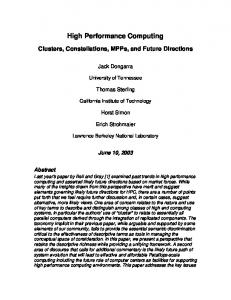
=1. 2.6 × 10 9 Interconnection network uses the QsNet, based on the Elan III network adapter and the Elite III switch. QsNet [31] has a fat-tree topology, as shown in figure 5 for a 128 node system, and offers a remote access latency of 2.5 µsec and a bandwidth of 210 Mbyte/sec. For a system with p nodes, granularity at the interval level is gm =

p ⋅ 2.6 × 10 9

≡ 12.4 . Granularity at the system p ⋅ 210 × 10 6 level has the same value, because both interprocessor communications and I/O operations are limited by the PCI speed.

Figure 5: fat-tree topology (128 nodes) An interesting comparison enlightening the better performances of QsNet with respect to the Gigabit Ethernet and Myrinet networks are reported in [41], where the MPI measured latency and bandwidth are given. In Table 1 we summarize such values. Table 1: Network Comparisons Bandwidth Latency (µs) (MB/s) Fast Ethernet 50 12.5 Gigabit Ethernet 15 125 Myrinet 20 62 QsNet 5 200 Network

6.3 Specialized system design In order to design specialized HW systems, we have developed a High Level Synthesis (HLS) methodology which, starting from a high level description of an affine iterative algorithm, allows its automatic hardware synthesis; theoretical basis of this approach can be found in [38],[39]. The HLS methodology is based on a sequence of steps which transform the high level description into

several lower level representations, until reaching the hardware implementation (described through a Hardware Description Language). Each transformation step is correct-by-construction, i.e. it preserve application semantics allowing the automatic implementation of the HLS methodology. In order to ensure the generation of correct-by-construction transformation steps, the algorithm high level description is given through a mathematical model of computation. In such a way each transformation step is mathematically proved to be correct. The chosen model of computation is the System of Affine Recurrence Equations (SARE) ([32] [33] [34]) which is one of the most promising model of computation in such fields arising in signal and image processing, linear algebra, scientific computing. SARE computational model allows the specification of an algorithm by means of recurrence equations.

7. Conclusions In this work a brief review of the supercomputer scenario has been presented, discussing advantages of custom vs commodity system implementation. Some theoretical aspects involved in heterogeneous system design and management have been introduced. Particular emphasis has been devoted to definition and discussions of task and system granularity. After underlying impact of a correct matching between task/system granularity, they were presented some results obtained in a scientific project aimed to exploit the advantages connected both to heterogeneity and to the use of custom parallel architectures. The outcome of this project was the PQE1 hybrid parallel system. After a brief description of its HW and SW environment, some examples of its use in several application domains have been reported (simulation of the sea level in the Venice lagoon, of the dynamic of galactic globular cluster, of electromagnetic field evolution). Finally, on the basis of the experience gained while developing this project, the HW/SW architecture of a next hybrid parallel prototype has been shortly presented.

Acknowledgments The authors acknowledge the fundamental role played by the Italian Project PQE2000 (which groups INFN, ENEA, CNR and QSW) for having triggered the idea of the PQE1 platform and for the collaboration during the course of the project. It should be emphasized the preminent role of M. Vanneschi, F. Baiardi, D. Guerri, M. Danelutto and S. Pelagatti (University of Pisa) in the realization of most of the SW structures (DVSM, SkIECL) which are supported by the PQE1 architecture and constitute its relevant assets. The role played by the QSW staff (R. Marega, B. Bacci, R. Castino, L. Di Iulio, S.

Pratesi, D. Rowet, A. Scippa, R. Simonazzi) in the platform realization is also acknowledged. The authors are also indebted to the staff of ENEA Funzione Centrale Informatica (INFO) for its constant technical support throughout the course of the project.

8. References [1] ALPHA 21264 Microprocessor Hardware Reference Manual [2] Accelerated Strategic Computing Initiative – ASCI – URL: http://www.sandia.gov/ASCI/ [3] Mathis, A.: Technologies for Teracomputing: a European Option. Para98 -Workshop On Applied Parallel Computing In Large Scale Scientific and Industrial Problems - Umea, Sweden June, 14-16, 1998 [4] The GRAPE project. URL: http://grape.c.utokyo.ac.jp/grape/ [5] Makino, J., Taiji, M.: Astrophysical N-body simulation on GRAPE-4 special purpose computer. Proceedings of Supercomputing 1995 [6] Makino, J.: Stellar dynamics on 200 Tflops special purpose computers. Proceedings of the International Symposium on Supercomputing (1997) [7] APE: The Italian SIMD supercomputer in the teraflop range. URL http://chimera.roma1.infn.it/ape.html [8] Battista, C. et al.: The APE100 Computer: (I) the Architecture. Int. Journal of High Speed Computing n. 5 –1993 [9] Bartoloni, A. et al.: The new wave of the APE Project: APEmille. Nucl. Phys. B, n. 42 – 1995 [10] Tripiccione, R. APEmille. Parallel Computing, vol. 25, n. 10-11, Oct. 1999, Special Issue: High performance computing in lattice QCD. [11] PQE1 prototype description - URL: http://www.pqe2000.enea.it/home/pqe1/PQE1_a.html [12] Vanneschi, M.: The PQE2000 Project on General Purpose Massively Parallel Systems''. Alta Frequenza, IEEE. November 1996. [13] Vanneschi, M.: PQE2000:HPC tools for industrial applications IEEE Concurrency, Vol 6, n.4, Oct-dec. 1998 [14] Pucello, N., Rosati, M., Celino, M., D'Agostino, G., Pisacane, F., Rosato,V.: Search of molecular ground state via genetic algorithm; implementation on a hybrid SIMD-MIMD platform, Lecture Notes in Computer Science; A.Bode, J.Dongarra, T.Ludwig, V.Sunderam Eds. (Springer) 1996 [15] Pucello, N., Celino, M., Rosato,V.: SuperComputing Application to Materials Science Engineering Proc. SIMAI 98 Conference, Giardini Naxos, Messina, Italy (1-5 June 1998) [16] Nicastro, S., Valentinotti, F.: An Atmosphere-Ocean Forecast System on a Hybrid Architecture. Proceedings of the Euromicro International Workshop on Parallel and Distributed Computing PDP 99. Madeira (Spain), 1999. [17] Valentinotti, F., Taraglio, S.: Phase Difference Stereo Disparity Computation on a SIMD Parallel Machine. Lecture Notes in Computer Science N.1225. Proceedings of High Performance Computing and Networking – Europe, HPCN'97, Vienna, Austria, April 1997. [18] Palazzari, P., Coli, M., Lulli, G.: Massively parallel processing approach to fractal image compression with nearoptimal coefficient quantization. Journal of Systems Architecture vol 45, n. 10, April 1999 pp. 765-779

[19] Palazzari, P., D'Atanasio, P., Ragusini, F.: Simulation of Patch Array Antennas by Parallel Finite-Difference TimeDomain Algorithm. Proceedings of the High Performance Computing and Networking – Europe (HPCN Europe 98), April 21st-23rd, 1998, Amsterdam (Nederland). [20] Palazzari, P., Adda, S., D'Atanasio, P.: A Tool for the Simulation of Electromagnetic Field Dynamic in Complex Environments through Massively Parallel Systems. 13th European Simulation Multiconference (ESM’99), Warsaw, Poland, June 1-4, 1999 [21] Coletta, M., Lippert, T., Palazzari, P.: Hyper-Systolic Implementation of BLAS-3 Routines in the APE100/Quadrics Machine. Para98 -Workshop On Applied Parallel Computing In Large Scale Scientific and Industrial Problems - Umea, Sweden June, 14-16, 1998 [22] Taraglio, S., Massaioli, F.: An efficient implementation of a Backpropagation learning algorithm on a Quadrics parallel supercomputer", Proceedings of the High Performance Computing and Networking – Europe (HPCN-Europe 1995), April 1995. [23] Gerasoulis,A., Yang,T.: On the granularity and clustering of directed acyclic task graphs. IEEE Transactions on Parallel and Distributed Systems, vol. 4, N. 6, Jun. 1993. [24] Meiko Web Page: www.meiko.com/info/TechnicalDescription/TechnicalDescripti on.html [25] Baiardi,F., Bernasconi,C., Guerri,D., Ricci,L., Vaglini,L.: Implementing concurrent paradigms through virtual shared areas. Technical report from Informatics Department, University of Pisa, November 1998. [26] Bacci,B., Cantalupo,B., Danelutto,M., Orlando,S., Pasetto,D., Pelagatti,S., Vanneschi,M. : An environment for structured parallel programming. In Advances in High Performance Computing, NATO ASI series e, Vol. 30, 1997. [27] Siegel, H. J., Maheswaran, M., Watson, D.W., Antonio, J.K., Atallah, M.J.: Mixed Mode System Heterogeneous Computing. Chapter 2 in the book ‘Heterogeneous Computing’, Ed. Eshigian,M.M., Arctech House, Norwood, MA, 1996. [28] Stone, H.S.: Multiprocessors. In High-Performance Computer Architecture, First Edition, Addison Wesley, 1987. [29] Bacci,B., Danelutto,M., Pelagatti,S., Vanneschi,M.: SkIE: A heterogeneous environment for HPC applications. Parallel Computing, Vol. 25, n.13-14, Dec. 1999. [30] Silbershatz, A., Galvin, P.B.: Virtual Memory. Chapter in Operating System Concepts, Addison Wesley, 1994 [31] www.quadrics.com/web/public/fliers/qsnet.html [32] Mongenet C.: Data Compiling for System of Affine Recurrence Equations. IEEE International Conference on Application - Specific Array Processors, ASAP, Aug. 1994. [33] Mongenet C., Clauss P., Perrin G.R.: Geometrical Tools to Map System of Affine Recurrence Equations on Regular Arrays. Acta Informatica, Vol. 31, No. 2, 1994. [34] Loechner V., Mongenet C.: Solutions to the Communication Minimization Problem for Affine Recurrence Equations. Proceedings of the EUROPAR ‘97, Passau, Germany, Vol. LNCS 1300, August 1997. [35] Sarkar, V. : Partitioning and scheduling parallel programs for multiprocessors. The MIT Press, 1989 [36] Lippert, T., Seyfried, A., Bode, A., Schilling, K.: HyperSystolic Parallel Computing. IEEE Trans. on Parallel and Distributed Systems, n. 1, 1998.

[37] Lippert, T., Glaessner, U. , Hoeber, H., Schilling, K. and Seyfried, A.: Hyper-Systolic Processing on APE100/Quadrics, in n2-loop computations'. Int. Jour. Mod. Phys. C, 7, 1996. [38] Marongiu, A., Palazzari, P.: A new memory-saving technique to map System of Affine Recurrence Equations (SARE) onto Distributed Memory Parallel Systems. International Parallel Processing Symposium IPPS99, April 1216, 1999, San Juan, Puerto Rico. [39] Marongiu, A., Palazzari, P.: Automatic Mapping of System of N-dimensional Affine Recurrence Equations (SARE) onto Distributed Memory Parallel Systems. Accepted to appear in the special issue of IEEE Trans. on Software Engineering on Architecture-Independent Languages and Software Tools for Parallel Processing [40] Saraceni, F., Coletta, M., Pucello, N., Rosato, V., Capuzzo-dolcetta,R.: On the use of a hybrid MIMD-SIMD platform to simulate the dynamics of globular clusters with an internal massive object. In preparation. [41] Allan, R.J., Guest, M.E.: Distributed Computing Programme.HPC Profile – The national publication for High – Performance computing applications and techniques, 24, pp1215, Dec. 1999

Paolo Palazzari, graduated in Electronic Engineering '89, Ph.D. '94. From '89 to '95 he was scientific assistant at the Electronic Engineering Department of University 'La Sapienza' in Rome. From '96 he is staff scientist at the Italian National Agency for New Technologies, Energy and the Environment (ENEA) where works on the High Performance Computing and Networking project. Main fields of his research are automatic parallelism detection for High Level HW/SW synthesis, routing, allocation and scheduling of parallel programs, image processing, neural networks and non linear optimization techniques. Lidia Arcipiani has a degree in Mathematics and a post-graduate “diploma” in Statistical Methodology. After ten years at the Electronic Division of the Italian Company Olivetti, she moved at the Italian Commission for Nuclear Energy (CNEN, now ENEA) as director of Casaccia Computing Centre. She has been acting as coordinator of computing, information and networking programs for the Department of Energy. At present she is staff scientist and R&D expert on the High Performance Computing and Networking Project of ENEA. She has been member of the National Committee for the Mathematical Science of the Consiglio Nazionale delle Ricerche (CNR) and vice-president of the National Committee for the Information Technologies of the CNR. She was professor of Computer Science at Catania University. Massimo Celino, graduated in Physics at the University "La Sapienza" of Rome (1992), has been working as Research Associate at the Department of Physics in the field of Statistical Physics. From 1994 he is working at the Italian National Agency for New Technologies, Energy and the Environment (ENEA). His work is mainly

focused on Computational Physics for applications in Materials Science and Quantum Chemistry. Other interests are in the field of computer programming and parallel algorithms for high performance computing platforms. Roberto Guadagni, graduated in Electronic Engineering at University “La Sapienza” of Rome in 1983. He is working at the Italian National Agency for New Technologies, Energy and the Environment (ENEA) from 1986. Now he is responsible of the supercomputing facilities in the Casaccia Research Center. Alessandro Marongiu, graduated in Electronic Engineering ‘95, Ph.D. 2000. Main fields of his research are automatic parallelism detection for High Level HW/SW synthesis, allocation and scheduling of parallel programs, cellular neural network design. Agostino Mathis is Director of the Interdepartmental Project "High Performance Computing and Networking" (HPCN) at the Italian National Agency for New Technology, Energy and the Environment (ENEA). He graduated in Electrical Engineering, and received a postgraduate "diploma" in Nuclear Engineering, at the Turin Polytechnic School of Engineering. He holds the "Libera Docenza" in Control Engineering at the Rome "La Sapienza" University. He is Professor of High Performance Computing at the Rome “Tor Vergata” University. He has published numerous papers on mathematical modeling of industrial processes, techniques for computer simulation, information systems for organizational management and high performance computing.

Paolo Novelli graduated in Physics at the University of Rome (Italy) in 1969. From 1971 to 1975, he was an assistant professor of electronics at the Physics Department of the same University. At the Italian National Agency for New Technologies, Energy and the Environment (ENEA) since the beginning of his professional activity, he was involved in the following fields: design of electronic devices for nuclear plants and analog computers, development of numerical models of uranium enrichment cascades, computational gasdynamics of ultracentrifuges. From 1982, he was involved in the corporate planning activities, and in 1987 he became the Head of the Organizational Development unit. In 1994, he came back to his past research interests and joined the High Performance Computing and Networking unit (HPCN). Vittorio Rosato, graduated in Physics at the University of Pisa (1979), received the Ph.D. at the University of Nancy (F) on 1986. He has been working as Research Associate at the University College of Wales in Aberystwyth (UK), at the Centre d'Etudes Nucleaires de Saclay (F), at the CECAM (Centre Europeen de Calcul Atomique et Moleculaire) in Orsay (F). From 1990 he is a Staff Scientist at the Italian National Agency for New Technologies, Energy and the Environment (ENEA). His research field is Computational Materials Science; in this area, he has been working on the development of interatomic potentials for metals and intermetallics and in their use to study thermodynamic and structural properties of complex materials. He is now active in the field of atomic-scale simulations of new C-based and Si-based materials. He is involved in design and realization of new tools (HW and SW) for HPC for scientific applications.