Simula Research Laboratory. P.O. Box 134, NO-1325 Lysaker, Norway. Email: {langguth,xingca}@simula.no. â . Department of Informatics, University of Oslo.
Heterogeneous CPU-GPU Computing for the Finite Volume Method on 3D Unstructured Meshes Johannes Langguth∗ and Xing Cai∗† ∗ Simula
Research Laboratory P.O. Box 134, NO-1325 Lysaker, Norway Email: {langguth,xingca}@simula.no † Department of Informatics, University of Oslo P.O. Box 1080 Blindern, NO-0316 Oslo, Norway Abstract—A recent trend in modern high-performance computing environments is the introduction of accelerators such as GPU and Xeon Phi, i.e. specialized computing devices that are optimized for highly parallel applications and coexist with CPUs. In regular compute-intensive applications with predictable data access patterns, these devices often outperform traditional CPUs by far and thus relegate them to pure control functions instead of computations. For irregular applications however, the gap in relative performance can be much smaller, and sometimes even reversed. Thus, maximizing overall performance in such systems requires that full use of all available computational resources is made.
the CPU and GPU sides, management of CPU↔GPU data transfers, invocation of computation on the GPU side, and synchronization between the two sides. For computations that are dominated by floating-point operations, a straightforward approach is to dedicate the CPU host exclusively to the above non-computational tasks, whereas the entire computation is offloaded to the GPU side. Such a GPU-only computing strategy is justified by the large difference in the floating-point capability between the two hardware types, and by the fact that the non-computational tasks can only be carried out by the CPU host.
In this paper we study the attainable performance of the cell-centered finite volume method on 3D unstructured tetrahedral meshes using heterogeneous systems consisting of CPUs and multiple GPUs. Finite volume methods are widely used numerical strategies for solving partial differential equations. The advantages of using finite volumes include built-in support for conservation laws and suitability for unstructured meshes. Our focus lies in demonstrating how a workload distribution that maximizes overall performance can be derived from the actual performance attained by the different computing devices in the heterogeneous environment. We also highlight the dual role of partitioning software in reordering and partitioning the input mesh, thus giving rise to a new combined approach to partitioning.
For computations whose performance is bound by memory bandwidth, which is the case for most scientific applications, the GPU-only computing strategy needs reconsideration. This is because the GPU-over-CPU advantage in memory performance is considerably smaller than the advantage in floatingpoint capability. Let us revisit the comparison between a K20 GPU and a Xeon E5-2650 CPU. The former has a peak memory bandwidth of 208 GB/s, whereas the rate is 51.2 GB/s for the latter. Moreover, the hardware data caches on a multicore CPU have a considerably larger capacity than those available on the GPU which makes it easier to achieve data reuse on the CPU. Therefore, if the CPU host includes some computational work in its responsibilities in addition to the non-computational tasks, the total computation time needed on a heterogeneous system may be considerably shortened.
I.
I NTRODUCTION
Graphics processing units (GPUs), together with coprocessors that are based on Intel’s many-integrated-core (MIC) architecture, are nowadays increasingly used as computing hardware. The main motivation is the tremendous computing power that these modern hardware units can deliver, in conjunction with an energy efficiency that is considerably higher than that of their multicore based CPU counterparts. For example, the Tesla K20 GPU from NVIDIA has a theoretical peak double-precision performance of 1.17 TFLOPS, i.e., 1.17×10¹² floating-point operations per second, whereas an 8core Intel Xeon E5-2650 2.0 GHz CPU has only 128 GFLOPS as its peak double-precision capability. Despite having a decisive upper hand in peak performance, GPUs rely on CPUs for delivering computing power. The current hardware architecture and programming paradigm chiefly treat GPUs as accelerators, which receive computational work from a CPU host. The CPU host itself can be made up of one or several multicore CPU chips. The responsibilities of a CPU host include allocation of data structures on both
However, a strategy of heterogeneous CPU-GPU computing requires more involved programming, in addition to introducing several questions: 1) 2) 3)
How much computational work should the CPU side handle? Which parts of the entire computation should be assigned to the CPU side? How can the non-computational tasks on the CPU host be arranged, so that these do not interfere with the assigned computation?
For computations that are based on structured computational meshes, the above questions are relatively easy to answer. This is mostly because the achievable performance on the CPU and GPU sides can be separately quantified by running a short sample of the target computation on the two different hardware platforms. This allows one to make an informed decision on which part of the computation should remain on the CPU side and which part should be offloaded
���������������������������������,(((
to the GPU. Moreover, the actual work division between the CPU and GPU sides is easy with such structured computations. There are several publications about heterogeneous CPU-GPU computation on structured meshes, such as [1], [2], [3], [6].
four neighboring tetrahedra, through the four triangular faces. Assuming the mesh is an approximation of a complex-shaped geometry, no structured way of ordering these tetrahedra exists in general, hence the term unstructured tetrahedral mesh.
In the case of unstructured meshes, however, the subject of heterogeneous CPU-GPU computing has been less studied. One particular difficulty is that the achievable performance on either hardware may not be easily quantified by a single sample execution. Changes in the mesh and/or the order of traversal can easily result in significant differences in performance. In addition to the challenge of deciding how much computational work should be assigned to the CPU side, there is the nontrivial issue of partitioning an unstructured mesh in order to achieve a desired load balance while limiting the amount of data transfer among all the involved hardware units. It is also more difficult to arrange the various tasks on the CPU side in connection with unstructured computations.
The following Eq. (1) is a representative computation for the cell-centered finite volume method on a 3D unstructured tetrahedral mesh. Its single-CPU or single-GPU performance is completely determined by the data traffic volumes at the different levels of the memory hierarchy between the registers and the memory, whereas the multi-device performance depends also on how data is distributed and communication is organized.
This paper investigates heterogeneous CPU-GPU computing in the context of the cell-centered finite volume method on 3D unstructured tetrahedral meshes. Extending our earlier work [7] on optimizing and modeling such unstructured computations on a single GPU, we aim to achieve resource-efficient exploitation of heterogeneous hardware systems that consist of a CPU host and multiple GPUs. As will be discussed in detail later, we need to first ensure an appropriate ordering of the tetrahedra, such that both hardware types can stably reach their realistically achievable performance. Then, the ordered tetrahedra are grouped into partitions and assigned to the accelerators and to the host. We investigate how the size of these partitions affects performance in the heterogeneous system and show a feasible way to obtain optimum load balancing in this setting. The remainder of this paper is organized as follows: We discuss the target finite volume computations in Section II and consider heterogeneous performance in general in Section III. Section IV describes the test implementation, Section V the experimental setup, and Section VI the experimental results. Finally, our conclusions are presented in Section VII. II.
C ELL - CENTERED FINITE VOLUME COMPUTATIONS
In this section we give a quick overview of cell-centered finite volume computations on 3D unstructured tetrahedral meshes, which constitute the context of our investigation of heterogeneous CPU-GPU computing. Finite volume computations using the GPU alone have been previously studied in various applications [8], [9], [10]. We also briefly summarize our earlier GPU-based work [7] to clarify the achievable performance of such 3D unstructured computations on CPUs and GPUs. These details are essential to develop the CPU-GPU work load division scheme presented in this paper. The cell-centered variant of the finite volume method solves partial differential equations by placing degrees of freedom at the center of each computational cell. Volume integrals that contain divergence terms are replaced with surface integrals, which as a result couple each pair of the neighboring cells. The 3D computational meshes we study are made up of tetrahedra, each having four triangular faces. The most common case is thus that each tetrahedron (except when lying on the boundary) is numerically coupled with exactly
y(i) =
4 �
A(i, j) (x(I(i, j)) − x(i)) . i = 1, 2, . . . , N, (1)
j=1
The vectors x and y contain two sets of the cell-centered degrees of freedom. The tetrahedron-tetrahedron couplings are stored in matrix A, which contains four weights per row, corresponding to the four neighbors per cell. The number of rows in matrix A is N , which represents the total number of tetrahedra in the mesh. Moreover, for each tetrahedron i, I(i, j) denotes the indices of its four neighboring tetrahedra, j = 1, 2, 3, 4. Since the overall computational mesh is unstructured, the indices returned by I do not in general have a recognizable pattern. In any computer program that implements Eq. (1), accessing the off-diagonal values x(I(i, j)) may result in randomly jumping back and forth in the 1D array that stores vector x. The accesses to the diagonal values x(i) and y(i), as well as the values of A and I, are always ordered. Good performance of any implementation of Eq. (1) thus relies on a suitable numbering of the tetrahedra, such that the jumps due to reading x(I(i, j)) can mostly be caught by some level of the hardware cache, without redundant memory reads. Let us perform a detailed analysis of memory traffic here. Suppose double precision is used for storing vectors x, y and matrix A, whereas values of I(i, j) are stored as integers. For computing each tetrahedron, at least (1 + 4) × 8 + 4 × 4 = 56 bytes have to be read from the memory, which accounts for the x(i), A(i, j) and I(i, j) values. Additionally, 8 bytes have to be written back to the memory for storing the newly computed y(i) value. That is, a minimum of 64 bytes per tetrahedron are transferred between the memory and the last-level cache. This minimum count assumes that all the off-diagonal entries x(I(i, j)) are kept in some level of cache. In the worst case, where none of the off-diagonal entries is cached, an additional 4 × 8 bytes per tetrahedron must be read from the memory, which translates to a 50% increase in memory traffic. Contrary to intuition, reordering the tetrahedra to minimize the bandwidth of the corresponding connectivity matrix may not be necessary to guarantee the best achievable performance, although such an approach does minimize the jumps within vector x caused by reading the off-diagonal x(I(i, j)) entries. We found in our earlier work [7] that it suffices to reorder the tetrahedra so that every b consecutive rows of the connectivity matrix are (mostly) contained within a b × b block. The size of b does not have to be extremely small. The threshold value of b for obtaining the best achievable performance depends on the target hardware. For example, to reach the realistically
achievable maximum performance for computing Eq. (1) on the K20m GPU, our experiments revealed the threshold value of b to be around 256. This number is mostly independent of the actual shape and size of the 3D unstructured mesh instances. For comparison, on the Xeon E5-2650 CPU we found that the threshold value of b was around 16000. This difference in threshold value is due to the CPU’s massive 20 MB L3 cache. In addition to the reordering, careful CPU and GPU implementations are required to minimize the amount of data loaded from the main/device memory of a CPU/GPU. Such implementations are be detailed in Section IV. However, note that even for careful implementations, the attainable memory bandwidth differs significantly from the theoretical peak memory bandwidth. It is tempting to use the following formula for estimating the best achievable performance for computing Eq. (1) in terms of floating-point operations per second: Performance =
Peak memory bandwidth × 11 . 64 bytes
Clearly, to minimize the time usage, the N CPU and N GPU values should satisfy the following relation: N CPU performanceCPU = . N GPU performanceGPU
(5)
Note that the accuracy of the realistically achievable values performanceCPU and performanceGPU , given by Eq. (3), depends on the tetrahedra being properly ordered into a blocked pattern of connectivity, and on using CPU and GPU implementations that take full advantage of the available memory bandwidths (see Section IV). Otherwise, the actual performance achieved will be highly variable and mesh-specific, making it impossible to determine beforehand an ideal CPU-GPU work division ratio as expressed by Eq. (5). Since N = N CPU + N GPU and the actual value of N is not relevant for load balancing, we can simplify the notation of work division by defining the accelerator load ratio r: r=
(3)
However, such an estimate still cannot be guaranteed to provide the realistically attainable performance since it disregards many of the complexities involved in the parallel computation. Therefore, in the following we use sample runs of the actual computation as a base of our performance estimates. III.
where N CPU is the number of tetrahedra assigned to the CPU side, and N GPU the number of tetrahedra on the GPU side, such that N CPU + N GPU = N . In Eq. (4), performanceCPU can be estimated by Eq. (3), in which the realistic memory bandwidth is an aggregate of all the involved CPU sockets. Similarly, performanceGPU can also be estimated by Eq. (3), considering the aggregate achievable memory bandwidth of all the involved GPUs.
(2)
In the above formula, the factor of 11 in the numerator corresponds to the 11 floating-point operations needed per tetrahedron, according to Eq. (1). The factor of 64 in the denominator is the minimum amount of data traffic in bytes that is transferred to or from memory. However, the estimate produced by (2) is too optimistic because the realistically achievable data transfer bandwidth is noticeably lower [12]. This is especially true when using Xeon Phi accelerators [11]. A simple memory benchmark, such as STREAM or similar, can be used to roughly quantify the realistic bandwidth on a target hardware. Given that, the achievable performance for computing Eq. (1) on a single device can be estimated Realistic memory bandwidth × 11 . Performance = 64 bytes
The time usage of a heterogeneous CPU-GPU computation of Eq. (1) can be expressed by the following formula: � � N CPU × 11 N GPU × 11 Time = max , (4) , performanceCPU performanceGPU
H ETEROGENEOUS PERFORMANCE
In this section we investigate the heterogeneous CPUGPU computation of Eq. (1) on 3D unstructured tetrahedral meshes. We assume that the CPU host is composed of one or more multicore CPU chips that share the system main memory. The GPU side of the heterogeneous hardware system consists of one or more accelerators. In such a heterogeneous scenario, maximum performance relies on three factors. First, the tetrahedra assigned to the CPU and GPU sides should all be properly reordered to exhibit a “blocked” connectivity pattern satisfying the respective threshold values of b, as discussed in the preceding section. Second, the numbers of tetrahedra that are assigned to the two sides should be balanced according to their respective performance capability, as detailed below. Third, the internal boundaries that result from the mesh partitioning should induce minimum CPU-GPU and GPU-GPU data exchanges.
N GPU . N
(6)
By substituting and transforming Eq. (5), we obtain the optimum value of r: ropt =
performanceGPU . performanceCPU + performanceGPU
(7)
The remainder of this paper is devoted to verifying the applicability of our load balancing model to the finite-volume computation in the form of Eq. (1) on 3D unstructured tetrahedral meshes. We only use GPUs of the same type for our subsequent experiments. However, the model can be easily extended to include multiple different types of accelerators. The crucial condition remains an equal ratio between performance and assigned work for each computing device. Similar to [4] and SWCWZ13, we have opted for a static work division scheme. While dynamic schemes are possible in principle, they do not interact well with the partitioning required by the unstructured mesh. Selecting tetrahedra at random and moving them to a different partition is likely to increase the size of the separator significantly, and thus incur large a communication cost. On the other hand, selecting suitable tetrahedra to avoid this or running the partitioner multiple times during the main computation is too slow to speed up the entire computation.
IV.
I MPLEMENTATION D ETAILS
Our hybrid CPU-GPU implementation aims to compute Eq. (1) for a prescribed number of iterations (or time steps). Between two iterations, vector x and vector y are swapped, i.e. time step t is computed from time step t − 1 only. Such iterations resemble scientific computations such as numerically solving diffusion equations. Given an unstructured 3D tetrahedral mesh, a pre-processing procedure is carried out to reorder the tetrahedra for obtaining a tetrahedrontetrahedron connectivity matrix that possesses a block pattern with b = 256. The hypergraph partitioner PaToH [13], [14] is used to achieve this goal by partitioning the original mesh into blocks of approximately 256 tetrahedra. However, the choice of partitioning software is not crucial for our results as there will always be a small number of connections that lie between the blocks. After the pre-processing procedure, the blocks are divided according to Eq. (6) and distributed to the CPU host and the GPUs. For each partition, we keep the separator, i.e., the set of tetrahedra that has neighbors in adjacent partitions, separate from the remaining tetrahedra and in a contiguous block. We refer to the tetrahedra that are not contained in any separator as the main set. Recall that the CPU side now has three main tasks: (1) invoking computation on the GPUs, (2) computing over the tetrahedra that are assigned to the CPU side, and (3) managing the CPU-GPU and GPU-GPU exchange of values that are required by the separators. Assuming that the CPU side has a shared main memory among the multicore CPU sockets, we choose OpenMP as the programming paradigm. For each GPU, one dedicated OpenMP thread is devoted to tasks 1 & 3 related to the GPU. The remaining OpenMP threads parallelize the computational work that is assigned to the CPU side.
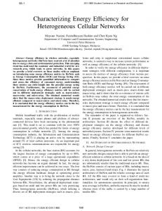
on the CPU host or by another GPU. We also use multiple CUDA streams to overlap communication with computation on the GPUs. That is, communication to and from the GPUs is mostly concurrent with the computation of the main tetrahedra set. At the end of each time step, the vectors x and y are swapped on both the CPU side and on the GPUs. Reorder tetrahedra into blocks of 256 Pack blocks into k partitions Partition 0 size is #tetrahedra * (1-r) Partition k size is #tetrahedra * (r/#GPUs) Split Partition k into separator SEP[k] and MAIN[k] #pragma omp parallel { if(computethread) { compute private separator_block_size move separator_block_size tetrahedra from SEP[0] into private arrays sep compute private main_block_size move main_block_size tetrahedra from MAIN[0] into private arrays main } if(controlthread) { Set device k Send Partition k separator tetrahedra to device k Send Partition k main tetrahedra to device k } for #timesteps do { if(computethread) { for each tetrahedron i in sep: computehost(i) set semaphore(threadid) for each tetrahedron i in main: computehost(i) } if(controlthread) { Set device k Stream 0: each tetrahedron i in SEP[k]: Launch computekernel(i) Stream 0: Send partial vector y(sep[k]) to host Stream 1: each tetrahedron i in MAIN[k]: Launch computekernel(i) wait for semaphores from all compute threads Stream 0: Send partial vector y to device }
A. A target heterogeneous system Our heterogeneous CPU-GPU system is equiped with two Intel 8-core E5-2650 processors running at 2 GHz and two NVIDIA K20m GPUs. Thus, out of the 16 available hardware threads, 14 are used for computation and 2 to control the GPUs. Using hyperthreading threads to control the GPUs yields no increase in performance. CPU threads are pinned on physical cores using the explicit KMP AFFINITY settings. This is necessary in order to obtain reproducible performance results. The two GPU control threads are split between the two sockets in order to equilibrate the number of active compute threads on each socket. Communication between the CPU cores residing on the same physical CPU socket utilizes the L3 cache and is thus extremely fast. On the other hand, communication between the two physical sockets using Quick path interconnect is much slower at 32 GB/s [15]. B. Hybrid CPU-GPU implementation An overview of the hybrid CPU-GPU implementation is given in Figure 1. For the sake of brevity, only the salient parts are shown in actual code, while the rest is shortened to pseudocode. The underlying principle is that values for the separator tetrahedra are computed first in each time step and then transferred to the CPU host. When the GPU→CPU transfers are completed, the host sends each GPU the separator values it requires, irrespective of whether they were computed
#pragma omp barrier #pragma omp master Swap(x,y) if(controlthread) { Set device k Swap(x,y) on device } unset semaphore(threadid) #pragma omp barrier } }
Fig. 1. Pseudocode for the heterogeneous implementation. The function computehost and computekernel are detailed below.
C. On the GPU side The actual computation on a GPU is performed by a CUDA kernel function that computes Eq. (1) for each tetrahedron in a straightforward manner while using the memory hierarchy efficiently. Details are given in Figure 2.
__global__ void computekernel (double* A, int* I, double* X, double* Y) { __shared__ double SM_A[Thread_Block_Size*4]; __shared__ int SM_I[Thread_Block_Size*4]; int b_start=blockIdx.x*blockDim.x*4 int tIdx = threadIdx.x; int i = threadIdx.x+blockIdx.x*blockDim.x; int l_x = threadIdx.x*4; SM_A[tIdx] =A[b_start+tIdx]; SM_A[tIdx+blockDim.x] =A[b_start+tIdx+blockDim.x]; SM_A[tIdx+blockDim.x*2]=A[b_start+tIdx+blockDim.x*2]; SM_A[tIdx+blockDim.x*3]=A[b_start+tIdx+blockDim.x*3]; SM_I[tIdx] =I[b_start+tIdx]; SM_I[tIdx+blockDim.x] =I[b_start+tIdx+blockDim.x]; SM_I[tIdx+blockDim.x*2]=I[b_start+tIdx+blockDim.x*2]; SM_I[tIdx+blockDim.x*3]=I[b_start+tIdx+blockDim.x*3]; __syncthreads(); Y[i] = SM_A[l_x+0]*(__ldg(&X[SM_I[l_x+0]])-__ldg(&X[i]))+ SM_A[l_x+1]*(__ldg(&X[SM_I[l_x+1]])-__ldg(&X[i]))+ SM_A[l_x+2]*(__ldg(&X[SM_I[l_x+2]])-__ldg(&X[i]))+ SM_A[l_x+3]*(__ldg(&X[SM_I[l_x+3]])-__ldg(&X[i])); }
Fig. 2. The CUDA kernel uses shared memory to accesses A and I in a coalesced manner.
As detailed in [16], the NVIDIA GK110 GPU, labeled K20m “Kepler” possesses 13 streaming multiprocessors, each equipped with 48 KB of read-only cache, as well as 64 KB of on-chip storage that is divided between shared memory and level 1 cache (L1). In our experiments 48 KB are assigned to shared memory. This cache works in a manner substantially different from a CPU, where the L1 cache does not need to be managed explicitly. On the other hand, the second level of cache (L2) on the GPU automatically caches all accesses to and from the GPU’s device memory. The K20m has 1280 KB of L2 cache which is shared among the 13 multiprocessors. Thus, it is comparable to the shared L3 cache on current multicore CPUs, except that it is much smaller. More powerful versions of the Kepler architecture, such as the K40 or Titan are available from NVIDIA. They have more streaming multiprocessors, a larger L2 cache, and a higher memory bandwidth, but otherwise work in the same way. In [7], several alternative kernels were tested for performance. For our purposes we use the most robust kernel, which uses shared memory to coalesce accesses to device memory. Thus, A and I are placed in the shared memory, while readonly cache is used exclusively for caching the x vector. Figure 2 shows the implementation details. Due to the comparatively large amount of memory traffic, the GPUs need to launch a large number of parallel threads in order to hide latency. Our kernel uses one thread per tetrahedron and a block size of 256 which mandates reordering the tetrahedra to be processed on the GPUs in blocks of exactly 256. However, setting the partitioner to produce blocks of exactly 256 tetrahedra might not yield good performance, since enforcing a strict size constraint might result in a proportionally large separator between the blocks, and thus inefficient use of the read-only cache in caching the x vector. We thus set the partitioner to create blocks having between 252 and 260 tetrahedra. Ideally, the partitioner would optimize the reordering by weighing the cost of underfull blocks against the cost of a large separator. However, current partitioners do not support this.
For our GPU kernel, the number of threads actually running in parallel is limited by the available shared memory. A thread block of 256 threads requires 256 ∗ 4 ∗ 8 = 8 KB of shared memory for A and half that amount for I, since the integer values require only 4 bytes each. Thus, only four such blocks (i.e., 1024 threads) can be run on a streaming multiprocessor in parallel with the available 48 KB of shared memory, even though the multiprocessor is theoretically capable of running 2048 threads at a time. D. On the CPU side Let blockstart be the first tetrahedron in the local block Let Loc_A be the local block of A Let Loc_I be the local block of I function computehost(tetrahedron i) { idx= 4*(i-blockstart); y[i] = Loc_A[idx]*(x[Loc_I[idx]]-x[i])+ Loc_A[idx+1]*(x[Loc_I[idx+1]]-x[i])+ Loc_A[idx+2]*(x[Loc_I[idx+2]]-x[i])+ Loc_A[idx+3]*(x[Loc_I[idx+3]]-x[i]); }
Fig. 3. Pseudocode for the multicore CPU compute implementation. Data from A and I is accessed
For the multicore part of the test platform, we use dual 8core Intel E5-2650 CPUs running at 2 GHz. Each core has 64 KB of L1 cache consisting of 32 KB instruction and 32 KB data cache, and 256 KB of unified L2 cache. Each processor also has 20 MB of L3 cache, which is shared among its cores. Unlike the GPU cache, the CPU cache is used automatically without explicit instruction by the programmer. However, using it to full effect still requires manual cache blocking. Since memory controllers are integrated in the processors, each CPU socket can access only its local memory at full memory bandwidth. The memory of the second socket must be accessed via the QuickPath Interconnect at higher latency, thus resulting in a non-uniform memory access (NUMA) architecture. The OpenMP CPU code is part of the heterogeneous implementation. Detailed code for the compute threads is shown in Figure 3. In preliminary experiments, we found that using a simple parallel for pragma is not sufficient for obtaining a scalable code in the NUMA environment. Thus, our implementation uses parallel regions in order to compartmentalize memory access to A and I, which can be beneficial in the NUMA environment and facilitates diverting some threads to control the GPU. Each CPU compute thread copies its relevant part of A and I into contiguous private arrays in the initialization step twice. Once for the separator, and once for the main part. We refer to these copies as the local block. The compute step code in Figure 3 works exclusively on local blocks. This code is the CPU equivalent of the GPU kernel described in Section IV-C, except that no explicit shared memory or cache management is performed here. Both initialization and computation are executed in the same parallel region, although the compute step is called multiple times. Since we use the parallel pragma instead of parallel for, the values of separator block size and main block size, i.e. the number of tetrahedra to be processed in each thread, must be computed explicitly. In our experiments this amounts to dividing work evenly among 14 threads, since the two remain-
ing threads are used to control the GPUs. The calculation is simplified in Figure 1. V.
E XPERIMENTAL S ETUP
In order to study the theoretically attainable performance, we use synthetically generated “ideal” instances to measure the impact of synchronization, communication, and load balancing in the heterogeneous environment. We then run our code on real world meshes in order to measure the realistically obtainable performance. Similar to [7], the synthetic instances are generated by ordering tetrahedra into tight blocks of 5 that are connected only among themselves. This is the smallest possible configuration since every tetrahedron can have 4 neighbors. Consequently, the values of x for the off-diagonal entries will always be in cache, which guarantees maximum single-device performance. There is no coupling between the blocks, but because 5 does not divide by 256, some of these blocks will be cut apart by the partitioner. Still, the resulting separators are very small and thus only incur a negligible additional communication overhead. Note that these synthetic instances do not correspond to any real mesh. They are constructed for performance testing purposes only. In our main experiments we use a mesh size of 10 million tetrahedra. Smaller test instances quickly lead to the CPU part of the problem fitting in cache entirely. In that case we obtain extremely high CPU performance which is not attainable in large scale real-world simulations. By avoiding small problems, we ascertain that our results are representative for all large problems. We also use some meshes containing one million tetrahedra to demonstrate this effect. The real world instances are obtained using the tetrahedral mesh generator Tetgen [17] on input structures available at the Tetgen website [18]. Our primary real world instance is the mesh brain, which is depicted in Figure 4(a). To obtain a varied test set, three secondary instances named body has heart, curvature 3 6, and hose n 2 6 were selected. The basic structure of these meshes is also shown in Figure 4. The meshes were refined in order to obtain a number of tetrahedra that is within 1% of 10 million. The main difference between the real-world and synthetic instances is the fact that the separators formed by the partitioner are much larger in the real-world instances. Note that the number of physical boundary tetrahedra does not affect the number of operations, and thus has no bearing on performance. All our GPU computations are performed on NVIDIA K20m Kepler GPUs with ECC turned off. Codes are compiled using nvcc 5.5. In order to obtain reliable performance measurements, 10000 time steps are executed for each run. However, usually only the first time step shows significantly lower performance, while all subsequent steps take approximately the same amount of time. Because 11 FLOPS must be performed to compute Eq. (1) for a single tetrahedron, overall performance can be calculated as N ∗10000∗11/runtime. We do not consider the time necessary for partitioning and initially transferring A, I, and x to GPU device memory, since this is done only once. In preliminary experiments, we determined the attainable performance when using either the CPU or the GPU
Fig. 4.
(a) brain
(b) curvature 3 6
(c) hose n 2 6
(d) body has heart
Test instances from the TetGen website [18].
alone. The maximum performance for each K20m GPU is about 27 GFLOPs. The dual E5-2650 processors yield about 11 GFLOPs together. This gives us an upper limit of 65 GFLOPs when using both GPUs and both CPUs on the test system, or 38 GFLOPs when using only one GPU. Of course, this performance can only be reached on an ideal test instance using optimal work division. Due to communication and synchronization cost, the actual heterogeneous performance will be lower. However, assuming that these effects slow down the CPU and GPU in equal proportions while using the above numbers, the optimum ratio ropt (real) of accelerator load using two K20m GPUs would be: 54 2 × 27 = = 0.83. (8) 11 + 2 × 27 65 Note that this formula does not require a specific unit of performance measurement such as GFLOPs. It can also be used with memory bandwidth values measured in GB/s. When using the peak memory bandwidth values of 208 GB/s per GPU and 51.2 GB/s per CPU, we obtain a value ropt (peak): ropt (real) =
ropt (peak) = VI.
416 2 × 208 = = 0.8. 2 × 208 + 2 × 51.2 518.4
(9)
E XPERIMENTAL R ESULTS
Our first experiment compares the attainable heterogeneous performance on the“ideal” synthetic instance with the realworld instance brain. In Figure 5, we show the result of this comparison with an instance size of 10 million tetrahedra. Both instances show the same performance when only the CPU is used. The performance curve for the synthetic ideal instance closely follows the GPU speedup limit line up to a value of r = 0.75. This limit is based on the fact that given the performance
of the CPU alone, for a given value of r the entire computation cannot be faster than the time it takes the CPU to compute its allotted workload, no matter how fast GPUs might be. Thus: performanceCPU . 1−r
(10)
In this region, the CPU is overloaded while the accelerator idles, and overall performance can be improved by increasing the accelerator load r. Once the GPU starts to become a limiting factor performance reaches a maximum. It then starts to decline when the CPU starts to idle. For the real world instance, we observe essentially the same behavior. However, for larger accelerator loads, i.e. r > 0.75, we notice a widening gap between both curves due to increased communication costs between the CPU and GPU. This communication is a result of using multiple compute devices at the same time. However, it has no noticeable influence on the optimum load balancing ratio. Thus, our model predictions remain valid. The performance maximum is indeed reached at r = 0.85, which is the closest point to the predicted r = 0.83 due to a resolution of r of 0.05 in Figure 5.
� �� ���������� �������� � �� ������ � � ������%�$#��������� &��
&�� %$� %�� $$� $�� #$� ��'�
��' �
��'!�
��'"�
��'#�
��'$�
��'%�
��'&�
��''�
��'(�
��(�
��� � � ���������� �� ������� ���� � ������� �
Fig. 6. 0.83.
� � �� �����
������ ����������
������ ����������
Performance and speedup limits around the optimum value of a =
In order to further investigate the similarity between the performance on synthetic and real meshes, we repeat the above experiment using three additional real-world meshes. Our results are shown in Figure 7. Even though the instances are unrelated, they show very similar performance due to the reordering step. Furthermore, all of the curves have essentially the same shape and peak at the same value of r. Therefore, we can use ropt (real) which was calculated using performance results gathered on an ideal instance in order to determine optimum load balancing for real-world meshes.
%��
������ � ��!���� �"�
�
������������ �� ����� &$�
� ����� �� ������� ��
GP U speeduplimit =
On the other hand, when using ropt (peak) as calculated in Eq. (9), i.e. r = 0.8, we incur a loss of about 11% or 6 GFLOPs of performance, which is larger than the contribution of one E5-2650 CPU.
$�� #�� "�� !�� �� ��� �� ��������#��������#��� ��� #���!���!#���"���"#���#���##���$���$#���%���%#���&���&#���'���'#�
�
���� ���������� ��� ������ ��� ����� ��
��������� ����� �������� ������� ���� ���
�������� ���� � ��
Fig. 5. Performance under varying accelerator load with instance size of 10 million tetrahedra.
In Figure 6, we repeat the above experiment at an increased resolution of r of 0.01. Clearly, the maximum performance is reached at r = 0.83, as predicted in our model. At this load balance ratio, the GPU speedup limit intersects with the analogously defined CPU speedup limit of 54 r , allowing for maximum performance. Note that due to the higher performance of the GPUs, the CPU speedup limit curve is flatter, and the real-world and synthetic instance performance follows this trend. Thus, if performance values are somewhat inaccurate, it is better to set r higher, i.e. towards the compute device with the higher performance. When using ropt (real) as calculated in Eq. (8), i.e. r = 0.83, the performance on the synthetic ideal instance amounts to 60.2 GFLOPs, which is close to the theoretical maximum of about 65. Thus, the overhead due to the synchronization of the devices is small. For the real-world instance, we attained 55.5 GFLOPs which is about 92% of the ideal instance value. It is also higher than the theoretical maximum of 54 GFLOPs, which could be obtained by using the two 27 GFLOP GPUs, assuming that no communication between them is necessary.
��������� �������� ��
���� �� � ����� ��
��� ��� ��� ��� ��� ��� �� ��������������������������������������������������������������������������� ��� ����!���!��
� ���������������� ���������� � �����
���� �
� �� �����
����� ��������
� ����� ����� �
Fig. 7. Performance under varying accelerator load for real-world instances.
Finally, we repeat the first experiment from Figure 5 with an instance size of one million tetrahedra. Results are shown in Figure 8. We immediately notice that maximum performance is not achieved using an accelerator load ratio of r = 0.83. Furthermore, the performance is even higher than the GPU speedup limit. This is due to the large L3 cache of the E5-2650 processors. With increasing accelerator workload ratio r, the CPU problem
� �� ���������� �������� � �� ������ � � ������$�#��������� &��
R EFERENCES [1]
������ � ��!���� �"�
%�� $�� #�� "��
[2]
!�� �� ���
[3]
�� ��������#��������#��� ��� #���!���!#���"���"#���#���##���$���$#���%���%#���&���&#���'���'#�
�
���� ���������� ��� ������� ���� �� � ����� ��
��� ����� ��
[4]
�������� ���� � ��
Fig. 8. Performance under varying accelerator load with instance size of one million tetrahedra.
[5]
size decreases and thus a progressively larger fraction of the CPU problem fits in cache, resulting in a superlinear speedup. This effect is noticeably smaller for the real world instance, because in this case communicated values will not be present in cache at the start of any given time step and thus take longer to be fetched from memory. While this effect could potentially be exploited in some cases by reducing the CPU workload ratio, most practical problems will be too large for the available L3 cache. However, it is necessary to keep this effect in mind when sampling performance. To avoid obtaining performance measurements that are based on L3 cache performance, large sample instances are needed, even though the number of time steps necessary to obtain a valid sample is small.
[6]
[7]
[8]
[9]
VII.
C ONCLUSIONS
We have investigated static work division for heterogeneous systems in the context of the cell-centered finite volume method. Due to a proper reordering of the tetrahedra, performance is stable over different unstructured instances. Thus, we can determine an optimum load balancing based on a performance sample of the compute devices on an idealized instance. On the other hand, we found that computing the load balancing based on the device’s peak memory bandwidth is not sufficient to obtain maximum performance. In fact, in our experiments this technique resulted in more than 10% performance loss. The method presented here can be used for many other scientific computations, provided that the performance can be sampled accurately. Mesh partitioning also plays a crucial role in this context on several tiers. At the first tier, partitioning data into cachesized blocks is crucial for performance. At the second tier, high-quality partitioning allows a load balancing distribution of the workload between the CPU and accelerators on a single compute node. This generally requires a partitioner that can create partitions of uneven sizes. In a multi-node environment, a third tier, i.e. even partitioning of the domain among the nodes is required. This is the classical application area of partitioners. While current state of the art partitioning software can be invoked multiple times to obtain such a multi-tier partitioning, it is currently very difficult to obtain a partitioning that is optimized simultaneously at multiple tiers.
[10]
[11]
[12]
[13]
[14]
[15]
[16] [17]
[18]
A. Humphrey, Q. Meng, M. Berzins, and T. Harman, “Radiation modeling using the Uintah heterogeneous CPU/GPU runtime system,” in Proceedings of the 1st Conference of the Extreme Science and Engineering Discovery Environment: Bridging from the eXtreme to the Campus and Beyond, ser. XSEDE ’12. New York, NY, USA: ACM, 2012, pp. 4:1–4:8. X. Yue, S. Shu, and C. Feng, “UA-AMG methods for 2-D 1-T radiation diffusion equations and their CPU-GPU implementations,” in 2013 21st International Conference on Nuclear Engineering. American Society of Mechanical Engineers, 2013, pp. V005T14A015–V005T14A015. M. Wen, H. Su, W. Wei, N. Wu, X. Cai, and C. Zhang, “High efficient sedimentary basin simulations on hybrid CPU-GPU clusters,” Cluster Computing, vol. 17, no. 2, pp. 359–369, 2014. S. Hampton, S. Alam, P. Crozier, and P. Agarwal, “Optimal utilization of heterogeneous resources for biomolecular simulations,” in High Performance Computing, Networking, Storage and Analysis (SC), 2010 International Conference for, Nov 2010, pp. 1–11. J. Chai, H. Su, M. Wen, X. Cai, N. Wu, and C. Zhang, “Resourceefficient utilization of CPU/GPU-based heterogeneous supercomputers for bayesian phylogenetic inference,” J. Supercomput., vol. 66, no. 1, pp. 364–380, Oct. 2013. T. Shimokawabe, T. Aoki, T. Takaki, T. Endo, A. Yamanaka, N. Maruyama, A. Nukada, and S. Matsuoka, “Peta-scale phase-field simulation for dendritic solidification on the TSUBAME 2.0 supercomputer,” in Proceedings of 2011 International Conference for High Performance Computing, Networking, Storage and Analysis, ser. SC ’11. New York, NY, USA: ACM, 2011, pp. 3:1–3:11. J. Langguth, N. Wu, J. Chai, and X. Cai, “On the GPU performance of cell-centered finite volume method over unstructured tetrahedral meshes,” in Proceedings of the 3rd Workshop on Irregular Applications: Architectures and Algorithms, ser. IA3ˆ ’13. New York, NY, USA: ACM, 2013, pp. 7:1–7:8. M. J. Castro, S. Ortega, M. de la Asunci´on, J. M. Mantas, and J. M. Gallardo, “GPU computing for shallow water flow simulation based on finite volume schemes,” Comptes Rendus M´ecanique, vol. 339, pp. 165 – 184, 2011. B. Hamilton and C. J. Webb, “Room acoustics modelling using gpuaccelerated finite difference and finite volume methods on a facecentered cubic grid,” Proc. Digital Audio Effects (DAFx), Maynooth, Ireland, 2013. M. Long and D. He, “Hydraulic erosion simulation using finite volume method on graphics processing unit,” in Information Engineering and Computer Science. ICIECS 2009., pp. 1–4. J. Fang, H. Sips, L. Zhang, C. Xu, C. Yonggang, and A. L. Varbanescu, “Test-driving intel xeon phi,” in The 5th ACM/SPEC International Conference on Performance Engineering. ACM, 2014. F. Duguet, “Kepler vs Xeon Phi : Nos mesures - et leur code source complet,” http://www.hpcmagazine.fr/en-couverture/ kepler-vs-xeon-phi-nos-mesures, June 2013. U. V. C ¸ ataly¨urek and C. Aykanat, “A hypergraph model for mapping repeated sparse matrix-vector product computations onto multicomputers,” in Proceedings of International Conference on High Performance Computing, Dec. 1995. ¨ V. C U. ¸ ataly¨urek and C. Aykanat, “A fine-grain hypergraph model for 2D decomposition of sparse matrices,” in Proceedings of 15th International Parallel and Distributed Processing Symposium (IPDPS), San Francisco, CA, April 2001. Intel Corporation, “An Introduction to the Intel QuickPath Interconnect,” http://www.intel.com/content/dam/doc/white-paper/ quick-path-interconnect-introduction-paper.pdf, Intel Corporation, Tech. Rep., January 2009. NVIDIA Corporation, “Nvidia’s next generation CUDA compute architecture: Kepler GK110,” Whitepaper, Tech. Rep., November 2012. H. Si, “TetGen. a quality tetrahedral mesh generator and threedimensional delaunay triangulator.” URL:http://tetgen.berlios.de, 2007. [Online]. Available: http://tetgen.berlios.de ——, “Tetgen: A quality tetrahedral mesh generator and a 3d delaunay triangulator,” http://wias-berlin.de/software/tetgen/.