Heuristic and Exact Algorithms for QoS Routing with ... - UTSA CS

IEICE TRANS. COMMUN., VOL.E85–B, NO.12 DECEMBER 2002

2838

PAPER

Heuristic and Exact Algorithms for QoS Routing with Multiple Constraints∗ Gang FENG† , Kia MAKKI† , Niki PISSINOU† , and Christos DOULIGERIS†† , Nonmembers

SUMMARY The modern network service of finding the optimal path subject to multiple constraints on performance metrics such as delay, jitter, loss probability, etc. gives rise to the multiconstrained optimal-path (MCOP) QoS routing problem, which is N P-complete. In this paper, this problem is solved through both exact and heuristic algorithms. We propose an exact algorithm E MCOP, which first constructs an aggregate weight and then uses a K-shortest-path algorithm to find the optimal solution. By means of E MCOP, the performance of the heuristic algorithm H MCOP proposed by Korkmaz et al. in a recent work is evaluated. H MCOP only runs Dijkstra’s algorithm (with slight modifications) twice, but it can find feasible paths with a success ratio very close to that of the exact algorithm. However, we notice that in certain cases its feasible solution has an unsatisfactorily high average cost deviation from the corresponding optimal solution. For this reason, we propose some modified algorithms based on H MCOP that can significantly improve the performance by running Dijkstra’s algorithm a few more times. The performance of the exact algorithm and heuristics is investigated through computer simulations on networks of various sizes. key words: QoS routing, multi-constrained path, additive QoS constraints, K-shortest-path algorithm, high-speed networking

1.

Introduction

Due to the increasing need for providing modern network services such as VoIP, video and interactive multimedia communications, quality-of-service (QoS) routing has attracted much attention in the past few years [20]. The major task of QoS routing is to identify a path or a tree that satisfies one or more QoS requirements. In case of unicast routing we need to find a path between a source and a single destination [3], while in case of multicast routing, we need to find a tree that spans a source and a group of destinations [17]. In terms of the responsibility of each node involved in the computing of the path (or the tree), QoS routing can also be classified into source routing [3] and distributed routing [21], [22]. In this paper, we restrict our interest to QoS unicast source routing, which means that Manuscript received October 11, 2001. Manuscript revised April 1, 2002. † The authors are with Telecommunications & Information Technology Institute, Florida International University, Miami, FL 33174, USA. †† The author is with the Department of Informatics, University of Piraeus, Piraeus 18534, Greece. ∗ This work is supported in part by NSF under grants No. 9810534, No. 9726253, No. 0196557 and No. 0123950, and the Greek GSRT under PENED grant.

the source node is going to take full responsibility for finding a qualified route to the given destination. We assume that a link-state routing protocol such as open shortest path first (OSPF) [18] is available to provide all necessary state information to the source node. QoS requirements are generally specified in terms of constraints imposed upon the corresponding performance metrics [23]. In [3], these constraints are roughly classified into link constraint and path constraint, and based on these concepts, the QoS unicast routing problems are divided into several categories, among which the path-constrained path-optimization (PCPO) problem and the multiple-path-constrained (MCP) problem are N P-complete [10] and have become a hot topic in the QoS routing community in recent years. Most previous works for the PCPO and the MCP problems only consider the cases when the number of constraints is small (≤ 2). For instance, as the most representative PCPO problem, the delay-constrained least-cost (DCLC) problem has received extensive studies, and consequently a number of exact and heuristic algorithms have been developed [7], [11], [13], [20]–[22], [25]. On the other hand, many researchers also studied the delay-cost-constrained (DCC) problem [2], [8], [12], which is an MCP instance with two constraints. For a complete overview of these algorithms published before the year of 2000, the readers are referred to [14]. In spite of the good performance of some of the prior works, in the past two or three years a few authors [7], [13], [14], [19] found that the heuristic algorithms based on the Lagrange relaxation are much more attractive either in the sense of the time complexity or from the quality of solution standpoint. For example, J¨ uttner et al. [13] and Feng et al. [7] almost at the same time proposed the same iterative algorithm for the DCLC problem, which is based on the linear Lagrange relaxation. The basic idea of this algorithm is to linearly combine the delay and the cost in terms of a parameter to form an aggregate weight w, and then use the Dijkstra’s algorithm [1], [4] to find the shortest path w.r.t. w. By tuning the parameter according to the path obtained in the previous iteration, the algorithm tries to find a good feasible path if there exists such one. Large quantities of experiments indicate that this algorithm can obtain the optimal† solution with

FENG et al.: HEURISTIC AND EXACT ALGORITHMS FOR QOS ROUTING

2839

a very high probability even when the network size is relatively large [7], and most importantly its time complexity is very low [7], [13]. Feng et al. further extended this algorithm to solve the DCC problem [8], and it also outperforms most existing algorithms. Our recent research results [9] demonstrate that, however, when the number of performance metrics considered is greater than two, e.g., the PCPO problem with two or more constraints or the MCP problem with three or more constraints, it is hard to develop efficient heuristic algorithms based on the linear Lagrange relaxation technique. Instead, the heuristic algorithm H MCOP proposed by Kormaz et al. [14], which is based on the nonlinear Lagrange relaxation, delivers much better performance. The difference between the linear and nonlinear Lagrange relaxation was illustrated in [14]. While the linear relaxation method might be trapped by an infeasible path, the nonlinear relaxation method can possibly search the whole feasible region. The major difficulty of the nonlinear relaxation lies in that we can not use Dijkstra’s algorithm to find a path that exactly minimizes the objective function. For more details, please see [14]. To attack this difficulty, H MCOP runs Dijkstra’s algorithm (with modifications) twice, one in reverse direction with linear relaxation and the other in forward direction with nonlinear relaxation. It has been proved through computer simulations that in case of two constraints H MCOP can outperform almost all known algorithms either in terms of the success ratio of finding feasible paths or in terms of the average cost of the obtained feasible paths. H MCOP was designed to solve the multiconstrained optimal-path (MCOP) problem, i.e., PCPO problem with multiple constraints. Despite of its excellent performance shown in [14] when compared with other heuristics, the “goodness” of the obtained solution is still unclear in comparison with an optimal solution. For this reason, we investigate the performance of H MCOP in this paper by comparing it with an exact algorithm in various situations. As a result, we propose two exact algorithms for the MCP problem and the MCOP problem, respectively. Previous works on the exact algorithms include the extended BelmanFord (EBF) algorithm [27] for the MCP problem and the A*Prune for the MCOP problem [16]. Compared with these algorithms, the exact algorithms described in this paper are easier to implement if one has a loopless K-shortest-path (KSP) algorithm ready for use. Computer simulations also demonstrate they are not very time consuming when the network size is not very large (e.g., ≤ 200 nodes). The second contribution of this paper is some modified algorithms based on H MCOP. Our experimental results indicate that even though the success ratio for finding feasible paths by H MCOP is very close to that of the exact algorithm, in certain cases the average

cost deviation between the obtained feasible solution and the optimal solution is not low enough to be satisfied. The modified algorithms described in this paper, however, can significantly improve its performance with slightly increased time complexity. The remainder of this paper is organized as follows. In Sect. 2, the MCOP problem is formally defined. In Sect. 3 two exact algorithms are described for the MCP and MCOP problems, respectively. A modified algorithm and its possible variants based on H MCOP are discussed in Sect. 4. The performance evaluation is given in Sect. 5, and Sect. 6 concludes this paper. 2.

Notations and Definitions

Since the modified algorithm to be proposed is based on H MCOP, most notations used in this paper are the same as in [14]. A network is represented by a digraph G(V, E), where V is the set of nodes and E is the set of links. Associated with each link e there are J nonnegative weights wj (e), j = 0, 1, · · · , J − 1 and a cost c(e). Each weight is corresponding to a constraint, and the upper bound of constraint j is denoted by Cj . A path is a sequence of non-repeated nodes p = (v1 , v2 , · · · , vk ) such that for a given 1 ≤ i < k there exists a link from vi to vi+1 . The notation e ∈ p means that path p passes through link e. The wj -weight and cost of path p are given by wj (e) and c(p) = c(e), wj (p) = e∈p

e∈p

respectively. By means of the above notations we define the multi-constrained optimal-path (MCOP) problem as follows. Definition 1: Given a routing request between a source s and a destination t, the multi-constrained optimal-path problem is to find a path p between s and t such that (i) wj (p) ≤ Cj , ∀j = 0, 1, · · · , J − 1 (ii) c(p) ≤ c(q) for any path q that satisfies (i). A path satisfying (i) is called a feasible path (or feasible solution), and otherwise an infeasible path (or infeasible solution). If a path satisfies both (i) and (ii), it is called an optimal solution. Without considering part (ii) in the above definition, the corresponding problem becomes the MCP problem, for which we are only concerned with the question whether there is a feasible path or not. In order to describe the exact algorithms for the † For the PCPO problem, there may exist more than one optimal solution. Therefore in this paper “the optimal solution” does not necessarily mean that there is only one optimal solution.


2840

MCP and MCOP problems in the next Section, we specially denote the shortest path between s and t w.r.t. wj by pj , and the least cost (LC) path by pc . 3.

Exact Algorithms for the MCP and MCOP Problems

As mentioned in Sect. 1, both the MCP problem and the MCOP problem are N P-complete. Thus, any exact algorithm for these problems generally can not be used in practical applications. However, an exact algorithm is very useful to evaluate the performance of other heuristic algorithms. In this Section, we describe two exact algorithms E MCP and E MCOP for the above two problems, respectively. Algorithm E MCP can find a feasible path for the MCP problem if there exists such one, while algorithm E MCOP can return the optimal path for the MCOP problem if there exists at least one feasible path. 3.1 Algorithm E MCP Our basic idea of the exact algorithm for the MCP problem is first to form an aggregate weight w(e) for each link e, and then use a loopless KSP algorithm [15], [26] to check the shortest paths w.r.t. w between s and t. Since the KSP algorithm can find the shortest path, the second shortest path, . . . , until there is no more path available between s and t, we definitely can find a feasible path as long as there exists at least one. The worst case is to enumerate all paths between s and t. The aggregate weight w(e) for link e is a linear combination of the J weights, given by w(e) = w0 (e) +

J−1

βj wj (e)

(1)

j=1

where βj , j = 1, 2, · · · , J − 1 are positive numbers. The reason to check the shortest paths w.r.t. the aggregate weight w instead of an individual weight is because by doing so we can possibly significantly reduce the number of paths to be checked before a feasible path is found or a conclusion of unavailability of a feasible path is reached. The above idea can be illustrated by a simple example. For the MCP problem described in Fig. 1(a), we assume that there are three paths between s and t,

(a) Fig. 1

(b)

A MCP problem with upper bounds of 5.

and there are three weights associated with each link (or path). The upper bounds of the three constraints are assumed to be 5. Obviously path q1 is the only feasible path. If we use a KSP algorithm to check the shortest paths w.r.t. any one of the three weights, path q1 must be the second shortest path. However, if we construct the aggregate weight w with β1 = β2 = 1, the w-weights of the three paths are shown in Fig. 1(b), from which we can see path q1 is the shortest path. There are two critical issues in the exact algorithm based on the above idea. First, what parameter should be chosen to construct the aggregate weight so that a feasible path can be found as early as possible? Second, when can we conclude that no feasible path is available? For a large network, there may have millions of paths between any two nodes. In that case, if there is no feasible path at all, definitely it is very time consuming and unwise to check all paths. Regarding the choice of parameters βj , j = 1, 2, · · · , J − 1, we recommend using the following method. Assuming that Cj ≥ wj (pj ), ∀j = 0, 1, · · · , J − 1, we first try to find a weight wj such that Cj > wj (pj ). If there does not exist such a weight (meaning Cj = wj (pj ), ∀j = 0, 1, · · · , J − 1), let βj = 1, ∀j = 1, 2, · · · , J − 1. Otherwise, without loss of generality we assume C0 > w0 (p0 ), and let βj be given by  ∞ : Cj = wj (pj )  βj = C0 − w0 (p0 ) : otherwise  Cj − wj (pj ) j = 1, 2, · · · , J − 1. For implementation, ∞ in the above formula can be replaced by a large number. The above method of choosing βj can ensure that the change of the aggregate weight has the equal effect on any constraint. This point is illustrated through Fig. 2, in which we assume there are two weights associated with each link, and hence we need to choose a value for β1 . Each black dot denotes a path with its w0 weight and w1 -weight being the horizontal and vertical coordinates, respectively. The shaded areas represent the feasibility regions. Any two paths located on the same contour line have the same value w.r.t. the ag-

(a) Fig. 2

(b) Search for a feasible path.


2841

gregate weight w. The KSP algorithm will return the path in the order being hit by the contour line sliding from the origin along the perpendicular direction. Figure 2(a) shows the case when β1 = 1, while Fig. 2(b) shows the case when β1 is computed by means of the method described above (assume β1 = 1 in the latter case). Since in the latter case the feasibility region is a square, the KSP can search at least half of the feasibility region before it returns an infeasible path, and thus significantly reduce the number of paths to be checked before a conclusion is made. One can imagine that in the case of more constraints, the feasibility region becomes a hypercube with equal length for each edge if βj is computed using the above method. Regarding the second question, we have the following proposition. Proposition 1: Given a path r, if w0 (r) + J−1 j=1 βj J−1 wj (r) > C0 + j=1 βj Cj , then r must be an infeasible path. Proof: If we assume that path r satisfies J − 1 constraints, then the remaining one must be violated. ✷ This proposition implies that M CPmax = C0 + J−1 j=1 βj Cj is the upper limit on the aggregate weight for a path to be feasible. When using the KSP algorithm to check the shortest paths one by one, if the wweight of the i-th shortest path exceeds M CPmax , we can conclude that all of the subsequent shortest paths must be infeasible. Based on the above analysis, we can develop an exact algorithm E MCP for the MCP problem. As shown in Fig. 3, this algorithm starts by finding the shortest path pj w.r.t. each weight wj , ∀j = 0, 1, · · · , J − 1. If Cj < wj (pj ) for any j, then the algorithm stops since it is impossible to find a feasible path. Otherwise, βj , w and M CPmax are computed based on our above description, and a loopless KSP algorithm is used to check the shortest paths w.r.t. w between s and t one by one. If the current shortest path r is a feasible path, then the algorithm terminates with r returned. If there is MCP(G(V, E), s, t, wj , Cj , j = 0, 1, · · · , J − 1) Find path pj , ∀j = 0, 1, · · · , J − 1. If (Cj < wj (pj )) for any j then return NULL /* no feasible path available */ Compute βj , ∀j = 1, 2, · · · , J − 1 Compute w(e) for each link e according to equation (1) J−1 β C set M CPmax = C0 + j=1 j j repeat r ←the current shortest path w.r.t. w found by a KSP algorithm 9 if (r = NULL) then 10 return NULL /* no more path */ J−1 β w (r) > M CPmax ) then 11 if (w0 (r) + j=1 j j 12 return NULL 13 if (wj (r) ≤ Cj , ∀j = 0, 1, · · · , J − 1) then 14 return r

E 1 2 3 4 5 6 7 8

Fig. 3

The exact algorithm E MCP for the MCP problem.

no more path between s and t, or if the w-weight of the current shortest path r exceeds M CPmax , we can also conclude that there is no feasible path. Otherwise, check the next shortest path. If the algorithm can not find a feasible path, a NULL pointer is returned. 3.2 Algorithm E MCOP The exact algorithm for the MCOP problem is based on the same idea as that for the MCP problem, i.e., we first construct an aggregate weight w(e) for each link e, and then use a loopless KSP algorithm to find the optimal solution. However, some details have to be changed since in this case we need to find a path with the minimal cost among all feasible paths. In order to take into account the cost c, the aggregate is given by w(e) = αc(e) + w0 +

J−1

βj wj (e)

(2)

j=1

where α and βj , j = 1, 2, · · · , J −1 are positive numbers. The parameters βj , j = 1, 2, · · · , J − 1 can be chosen in the same way as in the MCP case. Parameter α can be chosen as follows. If Cj = wj (pj ), ∀j = 1, 2, · · · , J − 1, we let α = 1. Otherwise, we assume that C0 > w0 (p0 ) and h is a feasible path with c(h) > c(pc ), and hence we let α be given by α=

C0 − w0 (p0 ) . c(h) − c(pc )

The way for choosing the value of α is based on the same philosophy as for choosing βj , i.e., to adjust all weights to the same level as w0 so that the change of the aggregate weight has almost the same impact on any constraint. Similar to the MCP case, for E MCOP we need to find a rule according to which we can judge whether there is a better solution or not. Regarding this issue, we have a similar proposition. Proposition 2: Assume that h is the best feasible solution obtained so far, and r is the current shortest J−1 path. If αc(r) + w0 (r) + j=1 βj wj (r) > αc(h) + C0 + J−1 j=1 βj Cj , then h must be the optimal solution. Proof: Assuming that r is a feasible solution, we must have c(r) > c(h), which means that path r is worse than h. ✷ With the above preparation, the exact algorithm E MCOP for the MCOP problem is described in Fig. 4. As we see, this algorithm first tries to find a feasible solution by means of algorithm E MCP without considering the cost c. If no feasible solution exists, the algorithm terminates, otherwise denote the feasible path by h. If c(h) = c(pc ), then the algorithm also terminates with h returned as the optimal solution. Otherwise,


2842 E MCOP(G(V, E), s, t, c, wj , Cj , j = 0, 1, · · · , J − 1) Step 1: Find a feasible path. 1 h ← E MCP(G(V, E), s, t, wj , Cj , j = 0, 1, · · · , J − 1) 2 if (h = NULL) then 3 return NULL 4 if (c(h) = c(pc )) then 5 return h Step 2: Find the optimal path. 6 Compute α 7 Compute w(e) for each link e according to equation (2) J−1 β C 8 set M COPmax = αc(h) + C0 + j=1 j j 9 repeat 10 r ←the current shortest path w.r.t. w found by a KSP algorithm 11 if (r = NULL) then 12 return h /* no more path */ 13 if (w(r) > M COPmax ) then 14 return h /* w(r) is given by equation (2) */ 15 if (c(r) < c(h) and wj (r) ≤ Cj , ∀j) then 16 h←r 17 update M COPmax Fig. 4

The exact algorithm E MCOP for the MCOP problem.

α, M COPmax and w are computed in accordance with the above description (note that βj , ∀j = 1, 2, · · · , J − 1 has the same values in E MCP and E MCOP). Subsequently, a loopless KSP algorithm is employed to check the shortest paths w.r.t. w one by one. If there is no more path between s and t, or if the w-weight of the current shortest path r is greater than M COPmax , then the algorithm terminates with path h returned as the optimal solution. If the current shortest path r is a feasible solution with a lower cost than h, then replace h by r, update M COPmax , and continue to check the next shortest path. 4.

A Modified Heuristic for the MCOP Problem

Most probably H MCOP [14] is so far the best heuristic algorithm for the MCOP problem, not only because of its low time complexity, but also due to its high success ratio of finding feasible solutions. In terms of the quality (cost) of the solution, it also considerably outperforms its predecessor TAMCRA [19]. In spite of this, in some cases its solution on average has a much higher cost than the corresponding optimal solution. In this section we describe a modified algorithm based on H MCOP that can significantly improve its performance with slightly increased time complexity. Before doing this, we describe a heuristic for the MCP problem which is also based on H MCOP. 4.1 Heuristic Algorithm H MCP As described in Appendix, H MCOP runs Dijkstra’s algorithm (with slight modifications on the relaxation procedures) twice: One in reverse direction with a linear cost function, and the second in forward direction

H MCP(G(V, E), s, t, wj , Cj , j = 0, · · · , J − 1) 1 Reverse Dijkstra (G(V, E), t, wj , j = 0, · · · , J − 1) 2 if (r[s] > J) then 3 return NULL /* no feasible path available */ 4 if (Rj [s] ≤ Cj , ∀j = 0, · · · , J − 1) then 5 return the path found by Reverse Dijkstra 6 Look Ahead Dijkstra(G(V, E), s, wj , Cj , j = 0, · · · , J − 1) 7 if (Gj [t] ≤ Cj , ∀j = 0, · · · , J − 1) then 8 return the path found by Look Ahead Dijkstra 9 return NULL Fig. 5

The heuristic algorithm H MCP for the MCP problem.

with a nonlinear cost function. Even though H MCOP can be directly used to solve an MCP problem by skipping all codes regarding the cost c, it does not achieve the best performance due to the particularity of the MCP problem. Given an MCP problem, we are only concerned with whether there exists a feasible solution or not. This differs from the case of solving an MCOP problem for which we need to find the best solution. Thus, if an algorithm for the MCP problem finds a feasible path, it may stop immediately with the path returned. For this reason, we may make slight modifications on H MCOP to obtain a heuristic algorithm H MCP for the MCP problem, which is shown in Fig. 5. Comparing Fig. 5 and Fig. A· 1 (in Appendix), one can see that H MCP is very similar to H MCOP. The major difference lies in that if a feasible path is found after calling Reverse Dijkstra, H MCP will stop and return this path (lines 4-5 in Fig. 5). Subroutine Reverse Dijkstra in H MCP, together with its relaxation procedure, is the same as that in H MCOP. Subroutine Look Ahead Dijkstra in H MCP is slightly different from the one in H MCOP in that the relaxation procedure for the former, which is shown in Fig. 6, does not contain those codes for processing the cost c (lines 2 and 7 in Fig. A· 3). For the same reason, procedure Prefer the best for H MCP shown in Fig. 7 is also slightly different from the procedure for the H MCOP shown in Fig. A· 4. Apparently, H MCP can achieve the same success ratio of finding feasible solutions as H MCOP does. However, unlike H MCOP which needs to run Dijkstra’s algorithm twice, H MCP could run only once if a feasible path is found by subroutine Reverse Dijkstra. 4.2 Heuristic Algorithm Modified H MCOP The pseudocode of heuristic Modified H MCOP is shown in Fig. 8. As we see, this algorithm is based on H MCOP and H MCP. Assuming that H MCOP returns a NULL pointer if no feasible path is found, Modified H MCOP first calls H MCOP to obtain an initial path r. If r is not NULL, then the MCOP problem is converted to an MCP problem with J + 1 constraints by setting cost c to weight J and c(r) − to the upper bound CJ of constraint J. is a small pos-


2843 Look Ahead Dijkstra Relax(u, v) 1 Let tmp be a temporary node 2a if λ < ∞ then g[tmp] =

J−1 j=0

Gj [u]+wj (u,v)+Rj [v] Cj

λ

2b

if λ = ∞ then Gj [u]+wj (u,v)+Rj [v] |0 ≤ j ≤ J − 1 g[tmp] = max C

3 4 5 6 7 8

Gj [tmp] = Gj [u] + wj (u, v) for j = 0, 1, . . . , J − 1 Rj [tmp] = Rj [v] for j = 0, 1, . . . , J − 1 if (Prefer the best(tmp, v) = tmp) then g[v] = g[tmp] Gj [v] = Gj [tmp] for j = 0, 1, . . . , J − 1 πg [v] = u

j

Fig. 6 The relaxation procedure of subroutine Look Ahead Dijkstra in H MCP.

Prefer the best (a, b) 1 if (∀j = 0, · · · , J − 1, Gj [a] + Rj [a] ≤ Cj ) then return (a) 2 if (∀j = 0, · · · , J − 1, Gj [b] + Rj [b] ≤ Cj ) then return (b) 3 if (g[a] < g[b]) then return (a) 4 return (b) Fig. 7

The preference rule used in H MCP.

Modified H MCOP(G(V, E), s, t, c, wj , Cj , j = 0, · · · , J −1) 1 r ← H MCOP(G(V, E), s, t, c, wj , Cj , j = 0, · · · , J − 1) 2 if (r = NULL) then 3 set wJ (e) = c(e) for each link e 4 set CJ = c(r) − ! 5 repeat 6 q ← H MCP(G(V, E), s, t, wj , Cj , j = 0, · · · , J) /*MCP problem with J + 1 constraints*/ 7 if (q = NULL) then 8 r←q 9 set CJ = c(r) − ! 10 until q = NULL 11 return r Fig. 8 The heuristic algorithm Modified H MCOP for the MCOP problem.

itive number such that no path between s and t has a cost in [c(r) − , c(r)]. H MCP is hence employed to solve the new MCP problem. Obviously if a feasible solution q is found by H MCP, q must have a lower cost than r. To further search for better solutions, we can replace r by q, update the upper bound CJ , and repeat this procedure until no feasible solution is found by H MCP. Modified H MCOP is an iterative algorithm. Other variants can be easily developed if one needs to firmly control the time complexity. For instance, we may restrict the number of times H MCP runs. In the extreme case, we may let H MCP run exactly once if a feasible solution is found by H MCOP, and thus the Dijkstra’s algorithm will be executed in total at most four times. Since Modified H MCOP (including the variants described above) starts from the solution of H MCOP, and considering that H MCP can obtain a feasible solution with a very high probability if such a path exists, Modified H MCOP can definitely surpass

H MCOP from the quality of solution standpoint. This will be demonstrated by the performance evaluation in the next Section. 5.

Performance Evaluation

In this Section, the proposed algorithms are tested on a number of randomly generated networks with random link weights. The experiments are designed in a way very similar to the one used in [14] in order to achieve a relatively fair comparison between H MCOP and our proposed modified heuristic algorithms. For this reason, Waxman’s method [24] used in [14] is also employed here to generate network topologies, even though there exist some other methods for modeling real communication networks [6]. We assume that in the following experiments there are three constraints. The three weights corresponding to the constraints are uniformly distributed on different sets of intervals, while the cost is always uniformly distributed on [1, 500]. Three types of networks (50-, 100- and 200node) are randomly generated. Given a network size and a set of intervals on which the link weights are distributed, a total number of 100,000 routing requests are generated as follows. First, 10 graphs are generated, then for each graph 10 instances of link weights are generated, and finally for each graph and each instance of link weights, 1000 routing requests are generated. To generate a routing request, a source and a destination are first randomly selected, then the shortest paths pj w.r.t. wj , j = 0, 1, 2 are computed via Dijkstra’s algorithm, and we let the upper bound Cj of each constraint j be given by Cj = γwj (pj ), j = 0, 1, 2 where γ is a positive number called constraint factor. For each routing request, both the exact algorithm E MCOP and the heuristics H MCOP and Modified H MCOP are employed to find a solution. Besides, two variants of Modified H MCOP, H MCOP MCP and H MCOP 2MCP, are also tested. H MCOP MCP restricts H MCP to be run exactly once if H MCOP returns a feasible solution, while H MCOP 2MCP restricts H MCP to be run at most twice. For all of these heuristics, the parameter λ used for nonlinear relaxation in procedure Look Ahead Dijkstra is fixed to be 25. For a specific algorithm, some of the following performance measures are computed based on its results for processing 100,000 routing requests on networks of a given size with link weights distributed on a specific set of intervals: • Success ratio (SR), which is the percentage of routing requests that feasible solutions have been found. One should be aware that H MCOP, Modified H MCOP and its variants have the same SR. • Success probability (SP), which is the probability


2844

Fig. 9

Performance measures with various values for γ.

that a heuristic can successfully find a feasible path if there exists at least one. It can be calculated in terms of SR as follows SP of heuristic H SR of heuristic H = . SR of algorithm E MCOP Similarly, H MCOP, Modified H MCOP and its variants must have the same SP. • Optimality, which is the probability that a heuristic can find the optimal solution if there exists at least one feasible path. If there are in total y routing requests for which there is at least one feasible path (found by E MCOP), and among them there are x routing requests for which heuristic H has found the optimal solution, then the optimality of heuristic H is given by x/y. • Average cost deviation (AvgDeviation), which is the average cost deviation in percentage between the feasible solution of a heuristic and the optimal solution.

In addition, other performance measures like the average number of executions of H MCP in Modified H MCOP are also computed. For some performance measures, 95% confidence intervals are provided as shown in the following figures and tables. 5.1 Performance Analysis with Different Values of Constraint Factor Assuming that the three link weights w0 , w1 and w2 are uniformly distributed on [1, 200], [100, 300] and [200, 400], respectively, we first analyze the performance when the constraint factor γ takes six different values between 1.25 and 2.5. The performance measures for each case are shown in Fig. 9. Figure 9(a) shows the average SR of the exact algorithm. According to our method for generating constraints stated above, we know that the larger the value of γ, the higher the probability that a feasible path exists. Thus, as shown in Fig. 9(a), the SR increases with the increase of γ. The SP of H MCOP is shown


2845 Table 1 γ 50-node 100-node 200-node

Average/maximum number of executions of H MCP with various values of γ.

1.25 1.03±0 / 4 1.03±0 / 3 1.02±0 / 3

1.5 1.16±0.03 / 5 1.2±0.01 / 6 1.17±0.01 / 4

1.75 1.34±0.05 / 5 1.42±0.04 / 6 1.42±0.01 / 6

in Fig. 9(b), from which we may conclude that in general H MCOP can find a feasible path with a very high probability if there exists one. The optimality of heuristics H MCOP, H MCOP MCP, H MCOP 2MCP and Modified H MCOP is shown in Fig. 9(c), from which one may notice that when γ is given a moderate value (e.g., 2), H MCOP MCP can achieve a much higher optimalH MCOP 2MCP and Modiity than H MCOP. fied H MCOP can further improve the optimality, but the improvements are less than the improvement between H MCOP and H MCOP MCP. However, with the increase of γ, the difference between the optimality of these heuristics becomes more and more conspicuous, and the number of executions of H MCP has to be increased to achieve better performance. Another observation is that for any heuristic the optimality decreases with the increase of γ. This is probably because the larger the value of γ, the more the feasible paths, and thus the harder the optimal solution can be found. The average quality of solution can be reflected by AvgDeviation as shown in Fig. 9(d). Once again we can see that Modified H MCOP and its variants can significantly reduce the cost deviation. For instance, when γ = 2.5 and the network size is 50, the AvgDeviation for H MCOP is about 60%, while it is below 10% for the modified algorithms. When Modified H MCOP is employed to process a routing request for which there exists at least one feasible solution, one may wonder how long it takes the algorithm to converge. The average and maximum numbers of executions of H MCP in such case are shown in Table 1. We notice that the average number of executions of H MCP is between 1 and 2 when γ = 2. This indicates that in most cases the major improvement of the performance of H MCOP is accomplished by the first run of H MCP. This complies with our previous observation that H MCOP MCP can considerably outperform H MCOP, while H MCOP 2MCP and Modified H MCOP can only improve the optimality by a little more than H MCOP MCP. However, with the increase of γ, the average number of executions of H MCP also increases and it is possible that H MCOP 2MCP makes a considerable improvement over H MCOP MCP, or Modified H MCOP over H MCOP 2MCP. Therefore one should carefully choose the number of executions of H MCP in order to make the best tradeoff between the time complexity and the performance.

2 1.5±0.02 / 6 1.62±0.02 / 6 1.64±0.02 / 6

2.25 1.63±0.02 / 6 1.76±0.02 / 7 1.84±0.03 / 7

Table 2

2.5 1.72±0.03 / 6 1.86±0.02 / 6 1.97±0.01 / 7

Three sets of link-weight intervals.

Set number w0 w1 w2

1 [1, 300] [1, 300] [1, 300]

2 [1, 100] [100, 200] [200, 300]

3 [1, 100] [1, 1000] [1, 10000]

Table 3 Average/maximum number of executions of H MCP with various sets of link-weight intervals. Set number 50-node 100-node 200-node

1 1.51±0.02/7 1.62±0.03/7 1.68±0.02/7

2 1.7±0.02/6 1.82±0.02/6 1.96±0.01/8

3 1.52±0.03/6 1.63±0.02/7 1.68±0.02/7

5.2 Performance Analysis with Different Sets of LinkWeight Intervals Now we investigate the performance of the heuristics when link weights are distributed on three different sets of intervals, which are enumerated in Table 2. In this case we let the constraint factor γ for each routing request be randomly selected from [1.2, 4]. Correspondingly, the performance measures are shown in Fig. 10 and Table 3. From Fig. 10 we can see that on one hand the heuristics can still achieve a very high SP, while on the other hand Modified H MCOP and the variants can still significantly outperform H MCOP in terms of the optimality or the average cost deviation. While we can see the link-weight intervals do affect the performance of these algorithms, they do not have substantial impacts. We notice that with the second set of link-weight intervals, it is more difficult for the heuristics to find the optimal solution in comparison with the cases with other two sets of link-weight intervals. This is due to the same reason as mentioned above, i.e., on average there are more feasible paths with the second set of link-weight intervals, as can be seen from the SR in Fig. 10(a). 5.3 Other Relevant Statistics Although the performance of the exact algorithms is not our major concern in this paper, some statistical results are also provided for future reference. Corresponding to the experiments in Sect. 5.1, Table 4 shows the average/maximum number of shortest paths checked by E MCP/E MCOP before a feasible/optimal solution is found or a conclusion is drawn that no feasible path is available, while these performance measures corresponding to the experiments in Sect. 5.2 are shown


2846

Fig. 10

Performance measures with various sets of link-weight intervals.

Table 4 Average/maximum number of paths checked by E MCP/E MCOP with various values of γ. γ 1.25 1.5 1.75 2 2.25 2.5

E MCP 5.78±0.54 / 4.82±1.57 / 3.31±1.23 / 2.44±0.57 / 1.91±0.33 / 1.57±0.27 /

50-node E MCOP 126 7.73±0.67 / 126 480 7.88±1.45 / 482 387 6.94±1.49 / 409 511 6.72±0.53 / 523 250 7.05±0.57 / 426 421 8.07±0.58 / 1041

100-node E MCP E MCOP 8.38±2.03 / 172 10.61±2.02 / 172 6.56±1.68 / 529 10.33±1.72 / 532 5.08±3.46 / 1690 9.63±3.7 / 1690 3.1±0.54 / 1557 8.6±0.77 / 1620 2.1±0.52 / 557 9.24±0.69 / 2462 1.65±0.27 / 323 11.27±0.94 / 1097

200-node E MCP E MCOP 15.53±1.98 / 246 17.85±1.94 / 246 15.68±2.85 / 2085 20.16±2.98 / 2102 11.97±1.98 / 6139 17.69±2.05 / 6139 9.08±2.77 / 4454 15.95±3.12 / 4454 5.47±1.8 / 4825 14.48±1.34 / 4830 3.47±1.58 / 8459 16.01±1.3 / 8500

Table 5 Average/maximum number of paths checked by E MCP/E MCOP with various sets of link-weight intervals. Set # 1 2 3

50-node 100-node 200-node E MCP E MCOP E MCP E MCOP E MCP E MCOP 1.79±0.12 / 33 14.3±3.33 / 15916 1.82±0.16 / 42 37.39±34.87 / 202028 2.28±0.15 / 45 30.4±4.66 / 30366 1.77±0.18 / 191 12.45±1.11 / 6044 2.04±0.26 / 510 23.47±7.61 / 67151 3.4±0.65 / 2571 43.69±8.59 / 105591 1.73±0.2 / 27 16.19±6.1 / 8062 1.83±0.17 / 41 28.99±7.28 / 33554 2.31±0.1 / 77 29.93±9.84 / 49791

in Table 5. Observing these data, we can see that for these experiments, in most cases (note the 95% confidence

intervals) E MCP only needs to check up to 20 paths, while E MCOP 80 paths. Even though these numbers are expected to increase with the increase of the net-


2847

6.

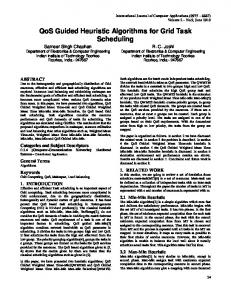
Fig. 11 The average time consumption of E MCOP and Modified H MCOP for processing 10,000 routing requests.

work size, it will not be very time consuming (on average) to find the optimal solutions even for a large number of routing requests on a network of a moderate size. Therefore, they may be very useful for evaluating other heuristics. However, we should also notice that the maximum number of paths checked by E MCP or H MCOP in some cases is extremely large. Therefore in the worst case the exact algorithms are still very time consuming and thus cannot be used in real-time applications. The actual computing times of the exact algorithm E MCOP and the heuristic algorithm Modified H MCOP are also obtained when these algorithms run on a Dell Pentium III computer. Figure 11 shows the average time the two algorithms need, respectively, to process 10,000 routing requests in the experiments in Sect. 5.1. One may notice that the computing time increases with the value of γ. This complies with our previous analysis as well as the statistical results in Table 1. One may also see that the average computing time of Modified H MCOP is much less than that of the exact algorithm. The computing time of other algorithms proposed in this paper can be estimated from the data shown in Fig. 11. For instance, under the same condition, the variants of Modified H MCOP should take less time than Modified H MCOP. Also, for a given routing request, on average E MCP needs much less computing time to find a feasible path than E MCOP needs to find the optimal solution. It should be pointed out that with different implementations of the KSP algorithm used in the exact algorithms, the computing time of E MCOP (or E MCP) may be different. Our implementation is based on the algorithm proposed in [5]. Since it is a not loop free algorithm, we have made slight modifications so that it only returns loopless paths.

Conclusions

As an important problem in QoS unicast routing, the problem of finding the optimal path subject to multiple constraints is studied in this paper. Both exact and approximate algorithms have been investigated for solving this problem. The proposed exact algorithm first constructs an aggregate weight for each link and then uses a K-shortest-path algorithm to search for the optimal solution. While in the worst case the exact algorithm has to check a large number of paths to identify the optimal solution or draw a conclusion, for the majority of experiments the number of paths to be checked is very small. Therefore, on one hand, the exact algorithm is not suitable for real-time applications, while on the other hand it is very useful to evaluate the performance of other heuristic algorithms. After making comparisons with the exact algorithm, we find that the heuristic algorithm H MCOP [14] can find a feasible path with a very high probability if there exists one. However, its optimality or average cost deviation from the optimal solution is not good enough. For this reason, we propose some modified heuristics based on H MCOP that can significantly improve the optimality with slightly increased time complexity. This is demonstrated by a large quantity of simulations on various networks with various link-weight intervals. A few variants of the modified heuristic can be developed to achieve the best tradeoff between the time complexity and the performance, enabling one to choose the most appropriate heuristic in a given situation. References [1] T. Cormen, C.E. Leiserson, and R.L. Rivest, Introduction to Algorithms, The MIT Press, 1985. [2] S. Chen and K. Nahrstedt, “On finding multi-constrained paths,” ICC’98, pp.874–879, Atlanta, GA, June 1998. [3] S. Chen and K. Nahrstedt, “An overview of QoS routing for next-generation high-speed networks: Problems and solutions,” IEEE Network, vol.12, pp.64–79, 1998. [4] E. Dijkstra, “A note on two problems in connexion with graphs,” Numerische Mathematik, vol.1, pp.269–271, 1959. [5] D. Eppstein, “Finding the k shortest paths,” SIAM J. Comput., vol.28, no.2, pp.652–673, 1998. [6] M. Faloutsos, P. Faloutsos, and C. Faloutsos, “On powerlaw relationships of the Internet topology,” ACM SIGCOMM’99, pp.251–262, Cambridge, MA, 1999. [7] G. Feng and C. Douligeris, “Fast algorithms for delayconstrained least-cost unicast routing,” shortened version presented in INFORMS’2001, Miami Beach, Nov. 2001, available at http://www.students.miami.edu/˜gfeng/ [8] G. Feng and C. Douligeris, “An efficient approximate algorithm for finding paths with two additive constraints,” IEICE Trans. Commun. (to appear). [9] G. Feng, Neural network and algorithmic methods for solving routing problems in high-speed networks, Ph.D. Dissertation, Univ. of Miami, 2001.


2848

[10] M.R. Garey and D.S. Johnson, Computers and Intractability: A Guide to the Theory of NP-completeness, W.H. Freeman and Company, 1979. [11] R. Hassin, “Approximation scheme for the restricted shortest path problem,” Mathematics of Operation Research, vol.17, no.1, pp.36–42, Feb. 1992. [12] J.M. Jaffe, “Algorithms for finding paths with multiple constraints,” Networks, vol.14, pp.95–116, 1984. [13] A. J¨ uttner, B. Szviatovszki, I. Mëcs, and Z. Rajk¨ o, “Lagrange relaxation based method for the QoS routing problem,” INFOCOM2001, vol.2, pp.859–868, Alaska, 2001. [14] T. Korkmaz and M. Krunz, “Multi-constrained optimal path selection,” INFOCOM2001, vol.2, pp.834–843, Alaska, 2001. [15] E.L. Lawler, Combinatorial Optimization: Networks and Matroids, Holt, Rinehart and Winston, 1976. [16] G. Liu and K.G. Ramakrishnan, “A*Prune: An algorithm for finding K shortest paths subject to multiple constraints,” INFOCOM2001, vol.2, pp.743–749, Alaska, 2001. [17] K. Makki, N. Pissinou, and O. Frieder, “Efficient solutions to multicast routing in communication networks,” Mobile networks and Applications, vol.1, pp.221–232, 1996. [18] J. Moy, “OSPF version 2,” Stands Track RFC 2328, IETF, April 1998. [19] H. Neve and P. Mieghem, “A multiple quality of service routing algorithm for PNNI,” Proc. ATM Workshop, pp.324–328, May 1998. [20] A. Orda and A. Sprintson, “QoS routing: The precomputation perspective,” INFOCOM2000, vol.1, pp.128–136, Israel, March 2000. [21] H. Salama, D.S. Reeves, and Y. Viniotis, “A distributed algorithm for delay-constrained unicast routing,” INFOCOM’97, vol.1, pp.84–91, Kobe, Japan, April 1997. [22] Q. Sun and H. Langendorfer, “A new distributed algorithm for supporting delay-sensitive applications,” Computer Communications, vol.21, pp.572–578, 1998. [23] Z. Wang and J. Crowcroft, “Quality-of -Service routing for supporting multimedia applications,” IEEE J. Sel. Areas Commun., vol.14, no.7, pp.1228–1234, 1996. [24] B.M. Waxman, “Routing of multipoint connections,” IEEE J. Sel. Areas Commun., vol.6, no.9, pp.1617–1622, Dec. 1988. [25] R. Widyono, “The design and evaluation of routing algorithms for real-time channels,” Tech. Rep. ICSI TR-94-024, University of California at Berkley, International Computer Science Institute, June 1994. [26] J.Y. Yen, “Finding the K shortest loopless paths in a network,” Management Science, vol.17, no.11, pp.712–716, July 1971. [27] X. Yuan and X. Liu, “Heuristic algorithms for multiconstrained quality of service routing,” INFOCOM2001, vol.2, pp.844–853, Alaska, 2001.

Appendix:

Heuristic Algorithm H MCOP

Figure A· 1 shows the heuristic algorithm H MCOP proposed in [14], which intends to find a path that satisfies a total number of J additive constraints. A cost function is defined in H MCOP as follows:

λ

λ w0 (p) w1 (p) gλ (p) = + + ··· C0 C1

λ wJ−1 (p) + CJ−1

H MCOP(G(V, E), s, t, wj , Cj , j = 0, 1, . . . , J − 1) 1 Reverse Dijkstra (G(V, E), t) 2 if (r[s] > J) then 3 return failure /* no feasible path available */ 4 Look Ahead Dijkstra(G(V, E), s) 5 if (Gj [t] ≤ Cj , ∀j = 0, 1, . . . , J − 1) then 6 return the path 7 return failure Fig. A· 1 The heuristic algorithm H MCOP for multi-constrained optimal path (MCOP) problem.

Reverse Dijkstra Relax(u, v) J−1 R [v]+w (u,v) 1 if r[u] > j=0 j Cj j then

J−1

R [v]+w (u,v)

2 3 4

r[u] = j=0 j Cj j Rj [u] = Rj [v] + wj (u, v) πr [v] = u

Fig. A· 2 Dijkstra.

The relaxation procedure of subroutine Reverse

where λ ≥ 1. The inputs of this algorithm include: a directed graph G(V, E) in which each link is associated with a primary cost c and J weights wj , j = 0, 1, . . . , J − 1, an upper bound Cj for each constraint, a source s and a destination t. The algorithm maintains for each node u the following labels: r[u], Rj [u], πr [u], g[u], Gj [u], πg [u], and c[u],j = 0, 1, . . . , J − 1. Label r[u] denotes the cost of the shortest path from u to t w.r.t. the cost function g1 , i.e., gλ with λ = 1. Labels Rj [u], j = 0, 1, · · · , J − 1 represent individually the accumulated link weights along that path. The predecessor of u along the path is stored in πr [u]. Label g[u] represents the cost of a complete path from s to t via node u w.r.t. cost function gλ (λ > 1). Labels Gj [u], j = 0, 1, · · · , J − 1 and c[u] represent individually the accumulated link weights and the primary cost from s to u along the path. The predecessor of u along the path is stored in πg [u]. Subroutine Reverse Dijkstra runs Dijkstra’s algorithm in a reverse direction with node t being the input value. The relaxation procedure used in this subroutine is shown in Fig. A· 2. One should notice that notation (u, v) denotes the link from u to v. As a result, Reverse Dijkstra can find the shortest path from every node u to t w.r.t. the cost function g1 (·). After the execution of Reverse Dijkstra, H MCOP checks the condition r[s] > J to judge if a feasible path exists based on a theorem proved in [14]. In case that the condition is false, H MCOP precedes to call subroutine Look Ahead Dijkstra, which runs the standard Dijkstra’s algorithm with a modified relaxation procedure described in Fig. A· 3. This subroutine starts with s and choose the next node based on the preference rule in Fig. A· 4. This rule will choose the next node that can lead to the primary cost being minimized if there exists a foreseen feasible path between s and t, and otherwise the cost function gλ (·) being minimized.


2849

Look 1 2 3a

Ahead Dijkstra Relax(u, v) Let tmp be a temporary node c[tmp] = c[u] + c(u, v) if λ < ∞ then g[tmp] =

J−1 j=0

Gj [u]+wj (u,v)+Rj [v] Cj

λ

3b

if λ = ∞ then Gj [u]+wj (u,v)+Rj [v] |0 ≤ j ≤ J − 1 g[tmp] = max C

4 5 6 7 8 9 10

Gj [tmp] = Gj [u] + wj (u, v) for j = 0, 1, . . . , J − 1 Rj [tmp] = Rj [v] for j = 0, 1, . . . , J − 1 if (Prefer the best(tmp, v) = tmp) then c[v] = c[tmp] g[v] = g[tmp] Gj [v] = Gj [tmp] for j = 0, 1, . . . , J − 1 πg [v] = u

j

Fig. A· 3 Dijkstra.

The relaxation procedure of subroutine Look Ahead

Prefer the best (a, b) 1 if c[a] < c[b] and (∀j, Gj [a] + Rj [a] ≤ Cj ) then return (a) 2 if c[a] > c[b] and (∀j, Gj [b] + Rj [b] ≤ Cj ) then return (b) 3 if (g[a] < g[b]) then return (a) 4 return (b) Fig. A· 4

The preference rule used in H MCOP.

After the execution of Look Ahead Dijkstra, H MCOP will return the feasible path recovered from labels πg [·] if such a path exists.

Gang Feng received his B.E. and M.E. from University of Electronic Science and Technology of China in 1992 and 1995 respectively, and Dr.Eng. from Beijing University of Posts and Telecommunications in 1998, all in electrical engineering. Between 1998 and 2001, he was studying in University of Miami, where he was granted Ph.D. in December 2001. Since July 2001, he has been working in Telecommunications & Information Technology Institute at Florida International University as a Research Associate. His major research interests include routing in next generation broadband wired/wireless networks, optical networking, combinatorial optimization, neural networks and evolutionary computation.

Kia Makki received his Ph.D. in computer science from the University of California, Davis, and two M.S. degrees from The Ohio State University and West Coast University. He is currently a tenure professor with an endowed chair professorship at Telecommunications & Information Technology Institute in Florida International University. His technical interests include wireless and optical telecommunications. He has over hundred refereed publications and his work has been extensively cited in books and papers. He has been Associate Editor, Editorial Board Member, Guest Editor of several International Journals including Editorial Board Member of several telecommunication journals. He has been involved in numerous conferences as a Steering Committee Member, General Chair, Program Chair, Program ViceChair and Program Committee Member.

Niki Pissinou received her Ph.D. in Computer Science from the University of Southern California, her M.S. in Computer Science from the University of California at Riverside, and her B.S.I.S.E. in Industrial and Systems Engineering from The Ohio State University. She is currently as a tenured professor and the director of the Telecommunication & Information Technology Institute at FIU. She has published over hundred refereed publications and has received best paper awards. She has also coedited seven volumes and is the author of an upcoming book on wireless Internet computing. She has also served as a steering committee, general chair and program committee member of over hundred programs and organizational committees of IEEE and ACM sponsored technical conferences. She has also refereed for a wide variety of conferences and journals, and has served as a reviewer on NSF and NASA panel reviews including the KDI and ITR panels. She has been the editor of eight journals including IEEE TKDE and guest editor of seven journals. She has received seven achievements awards and an invited speaker and keynote speaker of conferences.


2850

Christos Douligeris was born in Melissopetra, Arcadia, Greece. He received his Diploma in Electrical Engineering from the National Technical University of Athens in 1984 and the M.S., M.Phil. and Ph.D. degrees from Columbia University in 1985, 1987, 1990 respectively. He has held positions with the Department of Electrical and Computer Engineering at the University of Miami, where he reached the rank of associate professor and was the associate director for engineering of the Ocean Pollution Research Center. He has also held visiting positions at the National Technical Univ. of Athens and the Univ. of Piraeus, Greece. He has served in technical program committees of several conferences. His main technical interests lie in the areas of performance evaluation of high speed networks, neurocomputing in networking, resource allocation in wireless networks and information management, risk assessment and evaluation for emergency response operations. He is an editor of the IEEE Communications Letters and the IEEE Network, a technical editor of the IEEE Communications Magazine, a technical editor of the IEEE Communications Magazine Interactive, an associate editor of Computer Networks, a senior member of IEEE, and a member of INFORMS (formerly ORSA) and the Technical Chamber of Greece. During the academic year 1999–2000 he worked in the National Greek Agricultural Foundation as a Senior Fulbright Scholar.