HEURISTIC DYNAMIC ASSIGNMENT BASED ON AIMSUN MICROSCOPIC TRAFFIC SIMULATOR Jaime Barceló1 and Jordi Casas 2 1
Dept.of Statistics and Operations Research, Universitat Politècnica de Catalunya Pau Gargallo 5, 08028 Barcelona, Spain,
[email protected] 2 TSS-Traffic Simulation Systems, Paris 101, 08029, Barcelona, Spain,
[email protected] ABSTRACT The deployment of ITS must be assisted by suitable tools to conduct the feasibility studies required for testing the designs and evaluating the expected impacts. Microscopic traffic simulation has proven to be the suitable methodological approach to achieve these goals. This paper discuses one of the most critical aspects of the dynamic simulation of road networks based on a microscopic approach, namely how it performs a heuristic dynamic assignment, the implied route choice models, and whether under certain criteria it can achieve a stochastic user equilibrium. 1. INTRODUCTORY REMARKS From an analytical point of view dynamic traffic assignment has been usually related to the concept of the dynamic user equilibrium problems. Some of the most successful approaches are inspired on the seminal paper by Friesz et al. 1993, that proposes a dynamic network user equilibrium model which equilibrates the disutilities of the temporal choices. To achieve such equilibrium they take the perspective “that the essential choices available to users of a transportation network –route choice and departure time – occur in time-varying environments and are made rationally”, and they conclude with the assumption that these rational choices can only be made if the disutilities of the alternatives are equilibrated. Two main approaches have been used to model these route choices. One based on a generalization of Wardrop’s fist principle of static traffic assignment, in which users try to optimize their route based on the current information, this approach describes the evolution of flows when users make route choice decisions based on experienced travel times, and it is usually known as a preventive or enroute assignment, it does not achieve a day-to-day equilibrium pattern, therefore it is considered a dynamic traffic assignment principle and not a true equilibrium. In the above referenced paper Friesz et al. propose an alternative generalization of Wardrop’s principle stated in the following terms: If, at each instant in time, for each OD pair, the flow unit costs on utilized paths are identical and equal ti the minimum instantaneous unit path cost, the corresponding flow pattern is said to be in dynamic traffic equilibrium. This approach, also known as reactive assignment, can be interpreted in terms that could correspond to users having access to a real-time driver information traffic forecasting system or, alternatively, as an approximation to a process by which traveler combine the experienced travel times with conjectures to forecast the temporal variations in flows and travel costs. In the above reference the dynamic equilibrium problem is formulated in the space of path flows hk(t), for all paths k∈ Ki, the set of feasible paths for the i-th OD pair at time t. The path flow rates in the feasible region Ω satisfy at any time t∈(0,T) the flow conservation and non-negativity constraints:
⎧⎪ ⎫⎪ Ω = ⎨h(t ) | h k (t ) = gi (t ), i ∈ I; h k (t ) ≥ 0⎬ ⎪⎩ ⎪⎭ k∈K i for almost all t∈(0,T)
∑
(1)
where I is the set of all OD pairs in the network, T is the time horizon, and gi(t) is the fraction of the demand for the i-th OD pair during the time interval t. The approaches assume that the optimal user equilibrium conditions can be defined as (Friesz et al. 1993): A temporal version of the static Wardrop user optimal equilibrium conditions, that can be formulated as:
1
⎧= u i (t ) if h k (t ) > 0 s k (t )⎨ ⎩≥u i (t ) Otherwise
for ∀k ∈ K i , ∀i ∈ I, for almost all t ∈ (0, t ) h k (t ) ∈ Ω
u(t ) = Min{s k (t )}
(2)
k∈K i
Where sk(t) is the path travel time on path k determined by the dynamic network loading. Friesz et al. 1993show that these conditions are equivalent to the variational inequality problem consisting on finding h*∈Ω such that:
[S(h ),h − h ] ≥ 0, ∀h ∈ Ω *
*
(3)
According to (Florian et al., 2001), a dynamic traffic assignment model consists of two main components: 1. A method to determining the path dependent flow rates on the paths on the network, and 2. A Dynamic Network Loading method, which determines how these path flows give raise to time-dependent arc volumes, arc travel times and path travel times In the Dynamic Network Loading, also known as Dynamic Network Flow Propagation, (Cascetta, 2001), “models simulate how the time-varying continuous path flows propagate through the network inducing time-varying in-flows, out-flows and link occupancies”. A wide variety of approaches, from analytical, (Wu, 1991; Wu et al., 1998a; Wu et al., 1998b; Xu et al., 1998; Xu et al., 1999), to simulation based, (Florian et al., 2001), have been proposed. In all them path flows are determined by an approximate solution to the mathematical model for the dynamic equilibrium conditions. The differences between the various referenced approaches lay in the discretization scheme used to solve (3), and the algorithmic approach to solve the discretized problem (i.e. projection algorithms, successive averages, etc.) and the dynamic network loading mechanism, analytical (Wu, 1991; Wu et al., 1998a; Wu et al., 1998b; Xu et al., 1998; Xu et al., 1999), or simulation based (Florian et al. 2001). 2. HEURISTIC DYNAMIC TRAFFIC ASSIGNMENT BASED ON MICROSCOPIC SIMULATION The assessment by simulation of ITS applications requires a substantial change in the traditional paradigms of microscopic simulation, in which vehicles are generated at the input sections in the model, and perform turnings at intersections according to probability distributions. In such model vehicles have neither origins nor destinations and move randomly on the network. The required simulation approach must be based on a route based microscopic simulation paradigm. In this approach, vehicles are input into the network according to the demand data defined as an O/D matrix (preferably time dependent) and they drive along the network following specific paths in order to reach their destination. In the route based simulation new routes are to be calculated periodically during the simulation, and a Route Choice model is needed, when alternative routes are available to determine how the trips are assigned to these routes. The key question that this approach raises is whether this simulation can be interpreted in term of a stochastic heuristic dynamic traffic assignment or not. We propose to investigate the answer to this question in the case of a microscopic simulation using AIMSUN (2003), a route based microscopic simulator (Barceló et al. 1995, 1998). This paper is more elaborated version of a previous research reported in Barceló and Casas 2002 and 2004, and Barceló 2004. This process can be interpreted in terms of an heuristic approach to dynamic traffic assignment similar to the one proposed by Florian et al. 2001, consisting on: 1. A method to determining the path dependent flow rates on the paths on the network, based on a Route Choice function, and 2. A Dynamic Network Loading method, which determines how these path flows give raise to time-dependent arc volumes, arc travel times and path travel times, heuristically implemented by microscopic simulation. The implemented simulation process, Barceló and Casas 2004, and Barceló et al. 1995, based on time dependent routes consists of the following procedure, whose conceptual diagram is depicted in Figure 1, is as follows:
2
Procedure heuristic dynamic assignment Step 0: Step 1:
Step 2: Step 3:
Step 4:
Calculate initial shortest path(s) for each O/D pair using the defined initial costs Simulate for a time interval ∆t assigning to the available path Ki the fraction of the trips between each O/D pair i for that time interval according to the probabilities Pk , k∈ K estimated by the selected route choice model. Update the link cost functions and recalculate shortest paths, with the updated link costs. If there are guided vehicles, or variable message panels proposing a rerouting, provide the information calculated in 2 to the drivers that are dynamically allowed to reroute on trip. Case a (Preventive dynamic assignment) If all the demand has been assigned then stop. Otherwise go to step 1. Case b (Reactive dynamic assignment) If all the demand has been assigned and the convergence criteria holds then stop. Otherwise: Go to step 1 if all the demand has not been assigned yet Or Go to step 0 and start a new major iteration
Network with performance functions
Time depen dent OD Matrices
sa(v(t)) (1) PATH CALCULATION AND SELECTION
Determine paths and time dependent Path flows
Network Loading problem: Simulate the t th time interval using as input the g
(2) DYNAMIC NETWORK LOADING
Determine the new link flows, link travel times, path trave l times, …
Yes STOP
Convergence criteria satisfied?
No
Figure 1. Concpetual diagram of the heuristic dynamic assignment Depending on how the link cost functions are defined, and whether the procedure is applied as one pass method completed when all the demand has been loaded, or it is applied as part of an iterative scheme repeated until certain convergence criterion is satisfied, it corresponds either to a “preventive” or en route dynamic traffic assignment, or to a “reactive” or heuristic equilibrium assignment. In the first case route choice decisions are made for drivers entering the network at a time interval based on
3
the experienced travel times, i.e. the travel times of the previous time interval, and the link cost function is defined in terms of the average link travel times in the previous interval. Alternatively a heuristic approach to equilibrium can be based on repeating the simulation scheme a number of times and defining a link cost function including predictive terms, as proposed by Friesz et al. 1993, Xu et al. 1999. This could be interpreted in terms of a day-to-day learning mechanism. 2.1 Shortest path computation During the simulation, the computation of shortest paths is activated at each time interval ∆t. The shortest path routine used is a variation of Dijkstra's label-setting algorithm (Dijkstra 1959) that provides as a result the shortest path tree for each destination centroid. This structure of the shortest path tree provides the shortest path from every section to a destination. The penalties associated with turning movements are taken into account. Therefore, the cost labels are attached to links instead of nodes, as is usual. The link candidate list is stored as a heap data structure. During each iteration of the algorithm, the link with the minimum value of cost is removed from the heap and all links connected backward are added to the heap in the correct position. The shortest path routine is based on link cost functions, which are evaluated/updated with the available data at the beginning of each time interval. Three type of costs functions are considered (see AIMSUN and TEDI, 2003): •
•
•
The Initial Cost Function, used at the beginning of the simulation when there is not yet simulated data gathered to calculate the travel times. In this case, the cost of each link is calculated as a function of the travel time in free flow conditions and the capacity of the link. There are two types of default initial cost functions. The first does not consider the vehicle types IniCostj, that is, all vehicle types have the same initial cost. The second considers the vehicle types IniCostj, vt , which means that there is an initial cost function per vehicle type. Whether to choose the initial cost function distinguishing per vehicle type or not is determined by the presence of reserved lanes in the network. By default, AIMSUN takes the initial cost function not considering vehicle types. However, if there are reserved lanes, it takes the initial cost function considering vehicle types. The Dynamic Cost Function, used when there is simulated travel time data available, that is when the simulation has already started and statistical data has been gathered. The default current cost for each section is the mean travel time, in seconds, for all simulated vehicles that have crossed the link during the last time data gathering period. As for the Initial Cost Function, there are also two types of default dynamic cost function. The first does not consider vehicle types DynCostj, which means all vehicle types have the same cost. The second considers all vehicle types DynCostj, vt , which means that there is a dynamic cost function per vehicle type. Whether to use the dynamic cost function distinguishing per vehicle type or not is determined by the presence of reserved lanes in the network. User Defined Cost Functions. The default cost functions, described above, are basically defined in terms of link travel times and don’t consider directly other wide variety of link costs, for example toll pricing, historical travel times representing driver’s experience from previous days, combinations of various link numerical attributes as for instance travel times, delay times, length and capacity, etc. Therefore, for each particular link, the user may choose between using Initial Cost Function or Dynamic Cost Function as the default cost function, or using any other cost function defined by the user using the function editor in AIMSUN when he wants to take into account other arguments represented by other link numerical attributes. The function editor allows the user to define any type of numerical function in terms of the most common mathematical functions and operators (+ , -, *, /, ln, log, exp, etc.), using as function arguments any numerical attribute of the objects in the simulation model, either with fixed values (i.e. link lengths, number of lanes, speed limit on the link, etc.) or values that change during the simulation (i.e. link average speeds, average travel times, average flows, etc.
The heuristic dynamic assignment can then be defined as follows: Step 0:
Calculate initial shortest path(s) for each O/D pair using the defined initial costs
Step 0.1: Initialization:
4
Evaluate Initial Cost Function per each link j: for each j∈ 1... L : Costj = InitialCostj Step 0.2: Apply Shortest Path routine: for each destination centroid d: Calculate Shortest Path Tree SPTd using Costj j∈ 1... L Step 0.3: Identify Shortest Path from Shortest Path Tree: for each O-D pair i (from origin centroid o to destination d) Add to Path(s) SPcon to Ki Step 1:
Simulate for a predefined time interval ∆t assigning to the available path Ki the fraction of the trips between each O/D pair i for that time interval according to the selected route choice model.
Step 1.1: Assignment of path probabilities: for each O-D pair i: Calculate Pk using Route Choice Model, where k∈ Ki Step 1.2: Simulate for a predefined time interval ∆t, generating the fraction of the vehicles between each O/D pair i for that time interval, selecting randomly the path according probabilities Pk , k∈ Ki Step 2:
Recalculate shortest path, taking into account the experimented average link travel times.
Step 2.1: Update Link Cost Functions: Evaluate Dynamic Cost Function per each link j: for each j∈ 1... L : Costj = DynamicCostj Step 2.2: Apply Shortest Path routine: for each destination centroid d: Calculate Shortest Path Tree SPTd using Costj j∈ 1... L Step 2.3: Identify Shortest Path from Shortest Path Tree: for each O-D pair i (from origin centroid o to destination d) Add to Path(s) SPcon to Ki Step 3:
If there are guided vehicles, or variable message panels proposing a rerouting, provide the information calculated in 2 to the drivers that are dynamically allowed to reroute on trip.
Step 4:
If all the demand has been assigned then stop. Otherwise go to step 1.
2.2 Route choice based on a day-to-day learning mechanism In this case the simulation is replicated N times and link costs for each time interval and every replication are stored and thus at iteration l of replication j the costs for the remaining l+1, l+2,…, L (where L=T/∆t, being T the simulation horizon and ∆t the user defined time interval to update paths and path flows) time intervals for the previous j-1 replications can be used in an anticipatory day-tojl day learning mechanism to estimate the expected link cost at the current iteration. Let s a (v ) be the current cost of link a at iteration l of replication j, then the average link costs for the future L-l time intervals, based on the experienced link costs for the previous j-1 replications is:
s
j ,l + i a
1 j −1 m,l +i (v ) = ∑ sa (v ); i = 1,...., L − l , (4) j − 1 m=1 5
The “forecasted” link cost can then be computed as: L −l L −l j , l +1 ~ (v ) = α i s aj , l + i (v ); where sa α i = 1, α i ≥ 0, ∀i; are weighting factors (5) i=0 i=0 The resulting cost of path k for the i-th OD pair is
∑
∑
~ S k ( h l +1 ) =
∑ ~saj,l +1 (v)δ ak
(6)
a∈ A
( )
~ l +1 where, as usually δak is 1 if link a belongs to path k and 0 otherwise. The path costs S k h are the arguments of the route choice function (logit, C-logit, proportional, user defined, etc.) used at iteration l+1 to split the demand g il +1 among the available paths for OD pair i. In the computational experiments discussed in this paper a simplified version consisting of a link cost function defined as: c itk +1 = λc itk + (1 − λ )c~itk
(7)
Where c itk +1 is the cost of using link i at time t at iteration k+1, and c itk and c~itk correspond respectively to the expected and experienced link costs at this time interval from previous iterations. 2.3 Route Choice Models In the proposed network loading mechanism based on microscopic simulation vehicles follow paths from their origins in the network to their destinations. So the first step in the simulation process is to assign a path to each vehicle when it enters the network, from its origin to its destination. This assignment, made by a path selection process based on a discrete route choice model, will determine the path flow rates. Given a finite set of alternative paths, the path selection calculates the probability of each available path and then the driver’s decision is modeled by randomly selecting an alternative path according to the probabilities assigned to each alternative. Route choice functions represent implicitly a model of user behavior, that emulates the most likely criteria employed by drivers to decide between alternative routes in terms of the user’s perceived utility (or, properly speaking, a disutility, or cost in the case of trip decisions) defined in terms of perceived travel times, route lengths, expected traffic conditions along the route, etc. The simulation experiments reported in this paper have been implemented in AIMSUN selecting the Logit, C-Logit and Proportional route choice functions from the default route choice functions available in the simulator. The Multinomial Logit route choice model defines the choice probability Pk of alternative path k, k∈ Ki, as a function of the difference between the measured utilities of that path and all other alternative paths:
Pk =
e θVk
∑ l∈K i
e
θVl
=
1+
∑
1
e θ(Vl − Vk )
(8)
l≠k
where Vi is the perceived utility for alternative path i (i.e. the opposite of the path cost, or path travel time), and θ is a scale factor that plays a two-fold role, making the decision based on differences between utilities independent of measurement units, and influencing the standard error of the distribution of expected utilities, determining in that way a trend towards utilizing many alternative routes or concentrate in very few routes, becoming in that way the critical parameter to calibrate how the logit route choice model leads to a meaningful selection of routes or not. A drawback reported in using the Logit function is the observed tendency towards route oscillations in the routes used, with the corresponding instability creating a kind of flip-flop process. According to our experience there are two main reasons for this behavior. The properties of the Logit function, which
6
and the inability of the Logit function to distinguish between two alternative routes when there is a high degree of overlapping. The instability of the routes used can be substantially improved when the network topology allows for alternative routes with little or no overlapping at all, playing with the shape factor of the Logit function and re-computing the routes very frequently. However, in large networks where many alternative routes between origin and destinations exist, and some of them exhibit a certain degree of overlapping the use of the Logit function may still exhibit some weaknesses. To avoid this drawback the C-Logit model, (Cascetta et al., 1996; Ben-Akiva and Bierlaire, 1999), has been implemented. In this model, the choice probability Pk, of each alternative path k belonging to the set Ki of available paths connecting the i-th OD pair, is defined by:
Pk =
e θ (V k − CF k ) θ (V − CF l ) ∑e l
(9)
l∈ K i
where Vi is the perceived utility for alternative path i, i.e. the opposite of the path cost, and θ is the scale factor, as in the case of the Logit model. The term CFk, denoted as ‘commonality factor’ of path k, is directly proportional to the degree of overlapping of path k with other alternative paths. Thus, highly overlapped paths have a larger CF factor and therefore smaller utility with respect to similar paths. CFk is calculated as follows:
⎛ L ⎞ CFk = β ⋅ ln ∑ ⎜⎜ 1 2 lk 1 2 ⎟⎟ l∈I rs ⎝ Ll Lk ⎠
γ
(10)
where Llk is the length of arcs common to paths i and k, while Ll and Lk are the length of paths l and k respectively. Depending on the two factor parameters β and γ, a greater or lesser weighting is given to the ‘commonality factor’. Larger values of β means that the overlapping factor has greater importance with respect to the utility Vi; γ is a positive parameter, whose influence is smaller than β and which has the opposite effect. The utility Vi used in this model for path i is the opposite of the path travel time tti, (or path cost depending on how has been defined by the user). Other option is the estimation of the choice probability Pk of path k , k∈ Ki, in terms of a generalization of Kirchoff’s laws given by the function
P = k
CP k
−α
∑ CP
l∈ K i
−α
(11)
l
where CPl is the cost of path l, α is in this case the parameter whose value has to be calibrated. 3. INITIAL K-SHORTEST PATHS At the beginning of the simulation, using the Initial Cost function, one shortest path tree is calculated per each destination centroid, so during the first interval all vehicles are assigned to the same alternative. In order to start considering more than one alternative, as a way to anticipate the assignment process, at the beginning of the simulation, k-shortest path tree are calculated. The problem of enumerating, in order of increasing length, the k shortest paths has received considerable attention in the literature, Bellman 1960, Dreyfus 1969, Fox 1973, Eppstein 1994,1999. The different algorithms to solve this problem Eppstein 1994, Eppstein 1999, Jimenez et al. 1999, Martins 1984, Martins et al. 1996, are based in, after computing the shortest path from every node in the graph, the algorithm builds a graph representing all possible deviations from the shortest path. Therefore, all k shortest path obtained as a result, use the same length arc, associated to a cost function, and in our case the calculation of the k shortest path has to anticipate the evolution of the arc costs considering the traffic flow assigned to each path.
7
The algorithm calculates every iteration a new shortest path until the number of shortest path available reaches the parameter MaxKSP. The figure 2 depicts the generic scheme of the algorithm that iteratively:
evaluates the cost function in each arc (first iteration the cost function is the travel time in freeflow conditions) calculates a new shortest path . determine the path flow (using an incremental loading procedure, described bellow) and update the flow in each arc
The components of this algorithm are:
Shortest Path Algorithm The computation of the shortest path corresponds a variation of Dijkstra’s label setting algorithm. Arc Cost Function α ⎛ ⎡v ⎤ ⎞ The cost of using arc a (sa(va))is a function of the flow in arc a va : s a (v a ) = tt 0 ⎜1 + β ⎢ a ⎥ ⎟ ⎜ ⎟ ⎣ca ⎦ ⎠ ⎝
Incremental Loading Algorithm The path flow rates in the feasible region Ω satisfy the conservation flow and non-negativity constraint (where the traffic demand of O-D pair i is denoted by gi). That is:
Ω = hki :
∑h
k∈K i
i k
= g i , i ∈ I ; hki ≥ 0
For each O-D pair i ∈ I and path iteration n
hki , evaluate the path flow assigned to path hki
k ∈ K i at
hki (n) :
hki (n) = hki (n − 1) + λ ( g i − hki (n − 1)) hli (n) = hli (n − 1) − λ (hli (n − 1)), l = 1...(k − 1) where λ = 1 n +1
Demand: OD Matrix
Determine Paths: Shortest Path algorithm
Evaluate Cost Functions
Determine Path Flow: Incremental Loading
Network with Cost Functions Sa(va)
Figure 2: Generic scheme of K-Shortest Path Algorithm The algorithm to calculate the k-shortest path can be stated as follows (n is the iteration index and k is the shortest path index): Step 0: Initialization : n=0 and k=1 Compute the k-th shortest path based on the free-flow travel times.
8
For each O-D pair i ∈ I, assign
hki (n) = g i
Step 1: Compute the flow va for each arc a:
v a = ∑ ∑ δ ai ,k hki i∈I k∈K i
where
⎧1, arc a belongs to path k of O - D pair i ⎩0, otherwise
δa = ⎨
Evaluate the cost function of each arc a (sa(va)). Step 2: k= k +1, n = n +1 Compute the k-th shortest path based cost function of each arc a (sa(va)). Incremental Loading: For each O-D pair i ∈ I, evaluate:
hki (n) = hki (n − 1) + λ ( g i − hki (n − 1)) for l = 1 to ( k − 1) hli (n) = hli (n − 1) − λ (hli (n − 1)), l = 1...(k − 1) where
λ = 1n + 1
Step 3: If k is equal to total number of shortest path MaxKSP then STOP Otherwise, return Step 1 The figure 3 depicts an example of 3 initial k –shortest paths, in the model of the Preston network.
4. COMPUTATIONAL RESULTS No formal converge proof can be given for the proposed heuristic dynamic assignment algorithm, since the heuristic network loading process based on microscopic simulation does not have an analytical form. A set of simulation experiments has been designed and conducted to explore empirically whether the described assignment process, depending on how it is implemented, can be associated to a heuristic realization of a preventive or a reactive dynamic assignment, assuming that a proper selection of a route choice model with the right values for the θ, β, γ or α parameters, depending on the model, should lead to the realization of some equilibrium. A way of measuring the progress towards the equilibrium in an assignment, and therefore qualify the solution, is the relative gap function, Rgap(t) , Florian et al. 2001, Janson, 1991, that estimates at time t the relative difference between the total travel time actually experienced and the total travel time that would have been experienced if all vehicles had the travel time equal to the current shortest path:
∑ ∑h Rgap(t) =
k
(t )[s k (t ) − u i (t )]
i∈I k∈K i
∑ g (t)u (t ) i
(12)
i
i∈I
Where ui(t) are the travel times on the shortest paths for the i-th OD pair at time interval t, sk(t) is the travel time on path k connecting the i-th OD pair at time interval t, hk(t) is the flow on path k at time t, gi(t) is the demand for the i-th OD pair at time interval t, Ki, is the set of paths for the i-th OD pair, and I is the set of all OD pairs.
9
The figures 4, and 5, 6 and 7, and 8 and 9 respectively, depict the test networks, and time evolution of the Rgap(t) function for various Route Choice functions, for the preventive, or en-route version of the assignment procedure, using a K-shortest path algorithm, for the test models of :
• • •
The borough of Amara in the City of san Sebastián in Spain. A model with 365 road sections, 100 nodes and 225 OD pairs. The model of Brunnsviken network in Stockholm. This model has 493 road sections, 260 nodes and 576 OD pairs. The model of the Preston City Centre in UK. The model has 1375 road sections, 188 nodes and 1156 OD pairs.
Figure 3. 3 initial k-shortest paths in Preston City centre Model In these figures Logit n, corresponds to the above defined Logit function with value n for the shape parameter θ, proportional corresponds to a path probability inversely proportional to the path cost. The expected role of the θ parameter in terms of the Rgaps function becomes evident in the combination of the logit function with the assignment procedure. Improper choices of the parameter values tend to produce a bang-bang effect consequence of the tendency to move most of the flow to the current shortest path, as the oscillations of the Rgap function show, while a more appropriate θ value (θ = 30 in Amara, or θ = 900 in Brunnsviken) not only smooths out significantly the Rgap oscillations but also shows that a path selection with acceptable path costs differences (a 10% in Amara and around a 1% in Brunnsviken. The figures 10 and 11, depict the time evolution of the Rgap function for the same logit route choice function, for the reactive version of he assignment procedure using the costs as defined in (1), at iteration k=20, and λ=0.25, 0.5 and 0.75 respectively, for θ values of 30 in Amara, and 900 in Brunnsviken. Rgap values tend almost to zero, as expected in equilibrium terms, and the variations for the various values of λ show that λ=0.75 is the best. A side result of the method explored in this paper is the guidance that the computational results provide assisting in the calibration of the θ or α parameters, depending on the route choice function selected, based on the assumption that, as far as the described assignment process, depending on how it is implemented, can be associated to a heuristic realization of a preventive or a reactive
10
dynamic assignment, a proper route selection should lead to a realization of some equilibrium, and the progress towards such equilibrium is measured in terms of the Rgap function..
Figure 4. AIMSUN model of Amara RGAP (Am ara)
60,00%
50,00%
LOGIT 30
40,00%
LOGIT 60
30,00%
LOGIT 90
20,00%
LOGIT 300
10,00%
PROPORTIONAL
29
27
25
23
21
19
17
15
13
11
9
7
5
3
1
0,00%
Figure 5. Time evolution of the Rgap fuction for various Route Choice functions for Amara model (Preventive case)
11
Figure 6. AIMSUN model of Brunnsviken network in Stockholm 70,00%
60,00%
50,00% LOGIT 1 LOGIT 60
40,00%
LOGIT 90 LOGIT 300 LOGIT 900
30,00%
LOGIT 3600 Prport ional
20,00%
10,00%
0,00% 7:05 AM
7:10 AM
7:15 AM
7:20 AM
7:25 AM
7:30 AM
7:35 AM
7:40 AM
7:45 AM
7:50 AM
7:55 AM
8:00 AM
8:05 AM
8:10 AM
8:15 AM
8:20 AM
8:25 AM
8:30 AM
Figure 7. Rgap function for Brunnsviken (Preventive case)
12
Figure 8. AIMSUN model of Preston City Centre
25,00%
20,00% Proportional 15,00%
LOGIT 60 LOGIT 90 LOGIT 300 LOGIT 900
10,00%
LOGIT 3600 5,00%
0,00% 1
2
3
4
5
6
7
8
9
10
11
12
13
14
15
Figure 9. Rgap for Preston (Preventive case)
13
0,12
0,1
0,08 l=0.25 l=0.5 l=0.75
0,06
0,04
0,02
0 1
2
3
4
5
6
7
8
9 10 11 12 13 14 15 16 17 18 19 20 21 22 23 24
Figure 10. Rgap for Amara (Reactive case)
0,3
0,25
0,2 l=0.25 l=0.5 l=0.75
0,15
0,1
0,05
0 1
2
3
4
5
6
7
8
9
10
11
12
13
14
15
16
17
18
Figure 11. Rgap for Brunnsviken (Reactive case)
14
5. CONCLUSIONS Assuming that the “dynamic equilibrium” exists the empirical results show that a proper time varying kshostest paths calculation, with a suitable definition of link costs, and adequate stochastic route choice functions, using a microscopic network loading mechanism, achieves a network state that can replicate acceptably the observed flows over the simulation horizon, and led to a reasonable set of used paths between OD pairs as the oscillations within a narrow band of the empirical Rgap function indicates. 6. REFERENCES AIMSUN and TEDI Version 4.2 User’s Manual, TSS-Transport Simulation Systems, 2003. Barceló, J., J.L. Ferrer, R. Grau, M. Florian, I. Chabini and E. Le Saux, (1995), A Route Based variant of the AIMSUN Microsimulation Model. Proceedings of the 2nd World Congress on Intelligent Transport Systems, Yokohama. Barceló, J., J.L. Ferrer, D. García, M. Florian and E. Le Saux (1998), Parallelization of Microscopic Traffic simulation for ATT Systems Analysis. In: P. Marcotte and S. Nguyen (Eds.), Equilibrium and Advanced Transportation Modeling, Kluwer Academic Publishers. Barceló, J. and J. Casas (2002), Heuristic Dynamic Assignment based on Microscopic Traffic Simulation. Proceedings of the 9th Meeting of the Euro Working Group on Transportation, Bari, Italy. Barceló, J. and J. Casas, (2004) Methodological Notes on the Calibration and Validation of Microscopic Traffic Simulation Models, Paper #4975, 83rd TRB Meeting, Washington. Barceló, J., (2004) Dynamic Network Simulation with AIMSUN, Proceedings of the International Symposium on Transport Simulation, Yokohama, August 2002, Edited by Kluwer, to appear Summer 2004. Bellman R., and R. Kalaba, On kth Best Policies. J. SIAM 8 582-588 (1960) Ben-Akiva, M. and M. Bierlaire (1999),Discrete Choice Methods and Their Applications to Short Term Travel Decisions, in: Transportation Science Handbook, Kluwer. Cascetta, E., A. Nuzzolo, F. Russo and A. Vitetta (1996), A Modified Logit Route Choice Model Overcoming Path Overlapping Problems, in: Proceedings of the 13th International Symposium on Transportation and Traffic Flow Theory, Pergamon Press Cascetta, E., 2001, Transportation Systems Engineering: Theory and Methods, Kluwer Academic Publishers,. Dreyfus S.E., An Appraisal of Some Shortest Path Algorithms. Op. Res. 17 395-412 (1969) Eppstein D., Finding the k Shortest Paths. In: Proc. 35th IEEE Symp. FOCS, pp.154 –165 (1994) Eppstein D., Finding the k Shortest Paths. SIAM J. Computing 28(2) 652 – 673 (1999) Florian, M., M. Mahut and N. Tremblay (2001), A Hybrid Optimization-Mesoscopic Simulation Dynamic Traffic Assignment Model, Proceedings of the 2001 IEEE Intelligent Transport Systems Conference, Oakland, pp. 120-123. Fox B.L., Calculating kth Shortest Paths. INFOR - Canad. J. Op. Res. And Inform. Proces. vol 11 nº 1 pp. 66-70 (1973) Friesz, T., Bernstein, D., Smith, T., Tobin, R., Wie, B. A variational inequality formulation of the dynamic network user equilibrium problem. Operations Research, 41:179-191, (1993).
15
Janson, B. N., 1991, Dynamic Assignment for Urban Road Networks, Transpn. Res. B, Vol. 25, Nos. 2/3, pp. 143-161. Jiménez V. M and A. Marzal, Computing the K Shortest Paths: a New Algorithm and an Experimental Comparison”. Proc. of the 3rd Int. Workshop on Algorithm Engineering, WAE'99, London, July 1999. Martins E. Q. V., An Algorithm for Ranking Paths that may Contain Cycles, European J. Op. Res. 18 (1984) 123-130 Martins E.Q.V.and J.L.E.Santos, A New Shortest Paths Ranking Algorithm. Technical report, Univ. de Coimbra, http://www.mat.uc.pt/~eqvm (1996) Wu J.H. (1991), A Study of Monotone Variational Inequalities and their Application to Nertwork Equilibrium Problems, Ph. D. Thesis, Centre de Recherche sur les Transports, Université de Montréal, Publication #801. Wu J.H., Y. Chen and M. Florian (1998a), The Continuous Dynamic Network Loading Problem: A Mathematical Formulation and Solution Method, Trans. Res.-B, Vol. 32, No. 3, pp.173-187. Wu J.H., M. Florian, Y.W. Xu and J.M. Rubio-Ardanaz (1998b), A projection algorithm for the dynamic network equilibrium problem, Traffic and Transportation Studies, Proceedings of the ICTTS’98, pp. 379-390, Ed. By Zhaoxia Yang, Kelvin C.P. Wang and Baohua Mao, ASCE, Xu Y.W., J.H. Wu and M. Florian (1998), An Efficient Algorithm for the Continuous Network Loading Problem: a DYNALOAD Implementation, in Transportation Networks: Recent Methodological Advances, Ed. By M.G.H. Bell, Pergamon Press. Xu Y.W., J.H. Wu, M. Florian, P. Marcotte and D.L. Zhu (1999), Advances in the Continuous Dynamic Network Problem, Transportation Science, Vol. 33, No. 4, pp. 341-353.
16