Branch and Bound algorithm [7, 8] was used to find the optimal order in which the conflicted processes access the critical section. Branch and bound algorithm ...
Heuristic scheduling algorithms to access the critical section in Shared Memory Environment Tahany A. Fergany Engineering Mahematics Departmenrt Faculty of Engineering Cairo University, Egypt.
Reda A. Ammar Computer Science Department University of Connecticut Storrs, CT 06269-3155, USA. Ali I. El-Desouky Computer & Control Department Faculty of Engineering Mansoura University, Egypt.
Mohamed M. Hefeeda Computer & Control Department Faculty of Engineering Mansoura University, Egypt.
Abstract
The cooperation of n processes to solve a problem is useful only if the partial results are efficiently exchanged between processes. Shared variables facilitate communication among the processes. But they must be protected from nondeterminism, which can result from concurrent access by more than one process at a time. In order to protect the shared variables from nondeterminism, the code that hnadles these variables is placed in a critical section [1, 6, 9]. The critcal section is a section of code which can be executed by only one process at a time and which, once started, will be able to finish without interruption. Unfortunately, accessing the critical section by different processes will create a serial bottleneck that can seriously impair the performance of the software. Since shared memory multiprocessors are becoming more important in commercial environment, it becomes necessary to schedule shared memory access in the most efficient way. The scheduling problem [2-5, 7, 8, 10, 11] is complicated by the fact that each branch of parallel structure resulted from the FORK operation includes the time to process the portion of the code before accessing the shared variables, the time to access to the shared variables, and the time to process the portion of the code after using the shared variables, which may all be different. In order to make optimization possible, it is necessary to have an approach to quantify the time costs of parallel computations. After that, the time cost of processes which require access to the critical section can be minimized by using a suitable scheduling methods. The computation structure model [9] is used to represent the detailed time cost of a parallel structure. It is assumed in this model that the underlying computer system has a finite number of processors with the same speed and they communicate with each other through a shared
In shared memory parallel processing environment, shared variables facilitate communication among processes. To protect shared variables from concurrent access by more than one process at a time, they placed in a critical section. Scheduling a set of parallel processes to access this critical section with the aim of minimizing the time spent to execute these processes is a crucial problem in parallel processing. This paper presents heuristic scheduling algorithms to access this critical section.
1 Introduction The increasing demands for faster computers have led to the availability of many parallel computers. It is hoped that the impracticable computationallyintensive applications will be practicable by their execution on highly parallel computers. A number of factors prevent the growth of parallel computing. First, the substantial investment in sequential programming tools that aid in program testing, execution profiling, and interactive debugging. Second, the lack of a single, predominant, parallel architecture. Third, the difficulty of developing efficient programs for parallel computers. This paper addresses one of the obstacles that hinders producing efficient parallel programs; that is accessing the shared variables. In parallel programs, parallelism is gained through process creation. One of the most common mechanisms proposed for creation of processes is FORK/JOIN mechanism [1, 9], where the FORK statement spawns several processes and JOIN statement is used to synchronize the termination of processes. The portion of program between the FORK and JOIN is called the parallel structure. The semantics of the parallel structure require that exactly those processes created by FORK operation terminate at the associated JOIN operation and no operations after JOIN can start until all processes created by FORK are completed.
1
first evaluates these algorithms by simulation programs and compares between them. Second, it presents a new algorithm which gives a better results.
memory. In the computation structure model, the lock nodes are used to obtain locks on shared data and unlock nodes are used for releasing these locks. These locks facilitate protection of the shared variables.
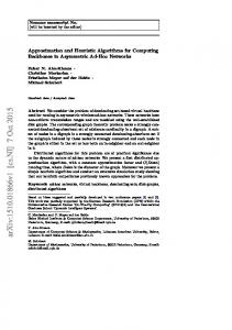
2 Previous Research Efforts Previously [2, 4, 7, 8], Algorithms were developed for accessing the critical section based on the time cost of the operations before the lock nodes, the time cost of the operations between the lock and unlock nodes, and the time cost of the operations after the unlock nodes. In the parallel structure in Fig. 1, assume that every two lock nodes are in conflict, and let: Time cost of the Pre-lock Job = PLJi Time cost of the Lock and Access Shared Variables = LASVi Time cost of the Remaining Job = RJi In order to schedule the operations between FORK/JOIN nodes (That are, the PLJs, the LASVs, and RJs) we considered eight possible cases which may arise in the parallel structure. These cases are listed in Table 1 along with their scheduling algorithms. In table 1, The “=“ indicates that all jobs have the same time cost; and ““ indicates that at least one job has a time cost different from the others. Algorithms for cases (I, II, III, IV, V, and VII) were mathematically proved to give the optimal solutions [7 ]. For cases VI, and VIII the Branch and Bound algorithm was developed which yields the minimum time cost for the parallel structure [7]. Although the Branch and Bound approach is widely acceptable technique [7], it is computationally expensive, especially when the problem size grows. So that heuristic algorithms were introduced which can produce optimal or near optimal solutions.
Fork
PLJ
LASV
RJ
B1
Bi
Bn
Lock1
Locki
Lockn
S1
Si
Sn
Unlock1
Unlocki
Unlockn
A1
Ai
An
Join
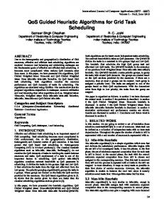
Fig. 1 Parallel structure model Join
In Fig. 1 we have a parallel structure with n branches that all are in conflict, i.e. they need to access the critical section simultaneously. In this parallel structure we can classify the operations into the following three categories: 1. The operation before accessing the critical section is defined as Pre-Lock Job, PLJ. 2. The operation of accessing the critical section which contains three sub-operations. These suboperations are: the lock operation to prevent other branches to access the critical section; the access of the shared variables operation; and the unlock operation to free the critical section for the other branches. So that, this combined operation is defined as Lock and Access Shared Variables, LASV. 3. The operation after accessing the critical section which is defined as Remaining Job, RJ. Algorithms were developed to schedule the access of the critical section [1, 6, 9 ]. Branch and Bound algorithm [7, 8] was used to find the optimal order in which the conflicted processes access the critical section. Branch and bound algorithm produces the optimal solution but it may take a long time to find it especially for large number of processes, greater than 8. So that, other heuristic algorithms were suggested [2, 4 ] which can produce optimal or near optimal solutions in short time. Those algorithms are called comparison and adjustment algorithms. This paper
Case
PLJ
LASV
RJ
Scheduling Algorithm
I
=
=
=
FCFS or LRJF
II
=
=
LRJF
III
=
=
FCFS or LRJF
IV
=
LRJF
V
=
=
FCFS
VI
=
Branch and Bound
VII
=
FCFS
VIII
Branch and Bound
FCFS: First Come First Served, LRJF: Longest Remaining Job First
Table 1 Scheduling Methods
2.1
Comparison Algorithm
A heuristic algorithm, i.e. not mathematically proved, that finds optimal solutions in some cases and near optimal solutions in the others. It is simple compared to Branch and Bound algorithm therefore it takes less time. For the parallel structure in Fig. 1
2
with n conflicted branches, the comparison algorithm is applied as follows:
reduce the execution time of the parallel structure. Move the maximum branch, the branch whose execution time is the longest, to the front of the waiting queue. In this way it can access the critical section earlier and hence its execution time reduces. Move the longest waiting branch, the branch that finishes its PLJ operation and waits the longest time to access the critical section, to the front of the waiting queue of the critical section. Thus, it can access the critical section earlier and reduces its execution time and the overall execution time. Simulation results, see section 4, showed that applying the new algorithm with the order: phase 1, phase 2, and finally phase 3 gave better results than the original algorithm. Moreover, when we changed the order of the phases to be phase 2, phase 1, and finally phase 3 the algorithm gave much better results. But another combinations of the three phases gave worse results than the original algorithm. We tried the following combinations: (phase 2, phase 3, phase 1); (phase 2, phase 3, phase 1, phase 3); (phase 1, phase 3, phase 2, phase 3); (phase 1, phase 2, phase 3, phase 2, phase 3) and all of them gave worse results.
1. Use the Longest Remaining Job First, LRJF, scheduling policy to order the branches of the given parallel structure. 2. If for every i = 2, 3, ... , n, PLJi-1 < PLJi, then the branches follows First Come First Served, FCFS, policy at the same time. No additional movements will be considered and the resulting order provides an optimal (or near optimal ) solution. 3. If for an i = 2, 3, ..., n, PLJi-1 > PLJi, and PLJi-1 - PLJi < RJi-1 - RJi , we reverse the order of the branch i-1 with branch i. 4. Repeat step 3 until no more movements.
2.2 Adjustment Algorithm The comparison algorithm is easy to apply but we need to add another round of adjustments to produce the optimal solution. the adjustment process is based upon the following two phases of movements: 1. Look for a branch that follows the current maximum branch and whose communication cost is smaller than the communication cost of a branch that precedes the current maximum branch. Swapping of these two branches may reduce the execution time of the parallel structure. 2. Move the maximum branch, the branch whose execution time is the longest, to the front of the waiting queue. In this way it can access the critical section earlier and hence its execution time reduces. This adjustment process is an iterative process and will continue until no more improvements is possible. The comparison algorithm is used to derive the initial solution for the adjustment algorithm.
3.1 Example: This example describes the application of the new algorithm on a parallel structure consists of five branches each branch has three time costs, PLJ, LASV, and RJ. The comparison algorithm is used to derive the initial solution. The following figure shows the application of the new algorithm. Initial solution 4 20 12
PLJ
92
83 LASV
55
71
67
68
54
3 The New Adjustment Algorithm
67
59
70
90
13
RJ
The adjustment algorithm produces optimal solutions in many cases and near optimal solutions in the others. Yet, we can add another round of enhancement, phase 3, which enhances the original adjustment algorithm and produces better results. Phase 3 states that: Moving the longest waiting branch, the branch that finishes its PLJ operation and waits the longest time to access the critical section, to the front of the waiting queue of the critical section may reduce the overall execution time. Thus, the new algorithm consists of the following three steps: 1. Look for a branch that follows the current maximum branch and whose communication cost is smaller than the communication cost of Apply phase 2 a branch that precedes the current maximum branch. Swapping of these two branches may After swaping branch 4 with branch 2.
134
197
275
363
340
Total Time Cost of each branch
Apply phase 2 Max. branch
3
12
4
92
20
83
55
71
68
67
54
67
59
90
70
13
134
197
296
343
340
12
20
92
4
83
After swaping branch 4 with branch 3.
�
�
�
55
67
68
71
54
67
70
90
59
13
134
204
292
332
340
0
47
42
198
190 Waiting time of each branch.
Apply phase 3
Longest waiting branch
4
20
92
12
83
71
67
68
55
54
59
70
90
67
13
134
212
300
332
332
different branches, and test to see if the new order is better than the previous one. b) If the new order has larger overall execution time then keep the previous order, and try another swapping. c) Evaluate the longest path of the parallel structure with the new order. Assume that the new maximum branch is branch k. d) If k = 1 or the execution time of the current parallel structure equals to the sum of execution times of PLJj, LASVj, and RJj, then the scheduling order we have is optimal and no additional improvement is possible. Otherwise, apply phase 1 again until no more improvement is achieved. 6. Apply Phase 3 as follows: a) Find the branch w that has the maximum waiting time. The waiting time of a branch x is evaluated by subtracting the time cost of PLJx of that branch from the time needed for the previous branch x-1 to finish the critical section. b) Initialize a displacement variable i to be 1. c) Swap the branch w with branch w-i. Evaluate the new execution time. d) If the new order has larger overall execution time then retrieve the previous order, increment i, and go to step 6.c. e) Evaluate the branch with maximum waiting time of the new parallel structure. Assume that the new branch is branch j. f) If j = 1 or the execution time of the current parallel structure equals to the sum of execution times of PLJj, LASVj, and RJj, then the scheduling order we have is optimal and no additional improvement is possible. Otherwise, apply phase 3 again until no more improvement is achieved.
After swaping branch 4 with branch 1.
Note that in the above figure, useless steps are omitted. The new adjustment algorithm can be written in steps as follows: 1. Find the branch k of the parallel structure, after applying the comparison algorithm, whose path has the longest execution time. 2. If k = 1, then the current parallel structure has the minimum possible execution time. 3. If the execution time of the parallel structure equals to the sum of execution times of PLJk, LASVk, and RJk, then the scheduling order we have is optimal and no additional improvement is possible. 4. Apply Phase 2 as follows: One)Initialize a displacement variable i to be 1. Two)Swap branch k with branch k-i. Evaluate the new execution times. Three)If the new order has larger overall execution time then keep the previous order, increment i, and go to step 4.b. Four)Evaluate the longest path of the parallel structure with the new order. If there is more than one branch has the same maximum value we use the back most one. Assume that the new maximum branch is j. Five)If j = 1 or the execution time of the current parallel structure equals to the sum of execution times of PLJj, LASVj, and RJj, then the scheduling order we have is optimal and no additional improvement is possible. Otherwise, apply phase 2 again until no more improvement is achieved. 5. Apply Phase 1 as follows: a) Set two pointers i (the front index) and j (the back index). The front index changes from 1 to k-1 and the back index changes from k+1 to n. For every value of j change i from 1 to k-1. If LASVi > LASVj then swap the two branches, evaluate the execution times of
4 Simulation Results This section, firstly, shows the effect of scheduling the critical section on the execution of parallel programs. Secondly, evaluates the scheduling algorithms and compares between them.
4.1 Effect of Scheduling To show the benefits of scheduling the access to the critical section, we developed a C++ simulation program. The program generates different number of branches, from 3 t0 8. For each branch, the program generates 500 sets of random values for PLJ, LASV, and RJ. Then, for each set it evaluates the execution time. Also, it finds the optimal order for the branches to access the critical section, this is done by trying all possisble permutations which equal the factorial of the number of branches. Then, it evaluates the optimal execution time. Eventually, it aggregates and averages the execution time and the
4
randomly. It starts with LASV range which is double the range of the PLJ and RJ until LASV range reaches only 1% of PLJ and RJ ranges; the last cases is likely to appear in practice. For each range, it generates different number of branches, from 3 to 8. For each branch it generates 500 sets of random values for PLJ, LASV, and RJ. Then, for each set it orders the branches according to the scheduling algorithm, Comparison, Adjustment, or New Adjustment, and evaluates the execution time. Then, it finds the optimal execution time by exhaustive search, i.e. trying all possible permutations which equal the factorial of no. of the branches, to compare with. If the optimal time is not equal to the time resulted after applying the algorithm, the program counts this case as a not-optimal one and evaluates the time difference between the time of optimal and not optimal cases. Then, it aggregates the time differences resulted from the not optimal cases out of the overall 500 cases. After that, the program evaluates the percentage of the total time difference to the total optimal time. The following pseudo-code describes the structure of the main body of the program.
optimal execution time over the 500 sets. The following pseudo-code describes the structure of the main body of the program. for( branches=3;branches