results, using RoboCup as an example domain, demonstrate the effectiveness of ... allow the use of single agent search algorithms such as A. â. [2] and IDA. â.
Proceedings of the 2006 IEEE International Conference on Robotics and Automation Orlando, Florida - May 2006
Heuristic Search for Coordinating Robot Agents in Adversarial Domains Ilya Levner, Alex Kovarsky, and Hong Zhang University of Alberta, Department of Computing Science, Edmonton, Alberta, T6G 2E8, CANADA,
Abstract— This paper presents a search-based, real-time adaptive solution to the multi-robot coordination problem in adversarial environments. By decomposing the global coordination task into a set of local search problems, efficient and effective solutions to subproblems are found and combined into a global coordination strategy. In turn, each local search entails the use of a heuristic evaluation function together with state space pruning to make the search tractable and scalable. Experimental results, using RoboCup as an example domain, demonstrate the effectiveness of the proposed framework on several simplified RoboCup scenarios.
I. I NTRODUCTION RoboCup is an international project designed to provide a common domain for research into Artificial Intelligence, Robotics and related fields. Although this paper is focused on the small sized soccer league sub-domain, in principle the framework is applicable to any multi-agent coordination task. While participating in RoboCup, we observed that many teams consistently miss obvious opportunities to control and advance the ball due, in our view, to a fundamental flaw in the structure of their AI, to which we refer as the ”handcoded” approach. Such approaches typically perform a static analysis of the field, e.g., examining the location of the ball and each robot, followed by an attempt to match the current field state to one of the hand-coded scenarios expected to occur during game play by the programmer. Once a match is found, the robots are commanded to move according to what the programmer thought would be a good response to the current situation. To reduce the complexity of the response, the programmer will naturally hand-code reusable behaviors such as covering a man, or getting open. In turn, such hand-coded behaviors achieve their objectives by using lower-level behaviors such as moving without hitting obstacles or dribbling the ball. This instinct to reduce complexity by layering reusable behaviors is a good one, but is fraught with problems. The first problem with the ”hand-coded” approach is that there is an infinite number of game situation predicates the programmer could think up, but only a (small) static set of these predicates can be realistically implemented. Second, each predicate prescribes a single response drawn from a large set of different immediate actions all the robots can execute in concert. Some teams, notably CMU [1], have used learning to find the best of a few possible responses. However, the chosen response or responses may not be the best possible. Indeed, it may be disastrous if the situation
0-7803-9505-0/06/$20.00 ©2006 IEEE
predicate happens to be satisfied by game states that do not resemble what the programmer imagined. In these cases the response can be extremely inappropriate. On the other hand, the major advantage of hand-coded AI is that it is easy for the programmer to get started and to continue adding capabilities. A. Heuristic Search Minimax search and its enhancements have been effective in perfect information games where two players alternate turns under moderate real-time constraints (e.g. chess). The alphabeta pruning [3] enhancement of minimax, can reduce the search time exponentially in its depth while still computing the correct minimax values and moves. Unfortunately, it is an alternating move algorithm, and therefore cannot correctly simulate simultaneous move execution within RoboCup. Monte Carlo Sampling (MC) is yet another technique for heuristic search. These methods search by executing a large number of (potentially biased) random actions and examining the numerical outcomes such actions generate. Such algorithms are usually employed for finding solutions to problems that are too complex to solve analytically. Unlike alpha-beta, Monte Carlo can simulate concurrent moves of both players since move selection decisions are made either randomly or pseudo randomly and thus are not influenced by opponent’s previous actions. Another possible advantage of Monte Carlo in real-time environments is the ability to distribute the workload and run the search in parallel on multiple machines, with results merged together afterwards. Unfortunately, the result of executing an action is non-deterministic when robots are used, and the number of actions a single robot can execute (let alone a team of robots) is immense. The large branching factor combined with non-deterministic actions implies that estimating the utility of the initial action being deliberated upon is intractable. Hence, real-time MC methods simply cannot (even partially) explore the huge state-space in a limited amount of time. One issue of applying two-player heuristic search to a domain such as RoboCup, is the difficulty in modeling the opponents’ actions. In the case the opponent team is unknown, which is usually the case, opponent modeling maybe totally impractical [1]. Assuming that the opposing team does follow certain heuristic actions, the search space can be pruned to allow the use of single agent search algorithms such as A∗ [2] and IDA∗ (Iterative Deepening A∗ ) [4]. To meet real-time constraints, the RT A∗ (Real Time A∗ [5]) extension uses
563
Minimin Lookahead to perform a fixed depth search and keeps track of moves leading to the heuristically best outcome, which are then propagated up the tree. In addition, to further reduce the utilization of limited resources, α-pruning is used to reduce the search effort. The minimum f-value at the leafs seen so far is called α, which is used for pruning interior nodes with values bigger or equal to α. RT A∗ then uses results from the minimin search as heuristic values in order to guide the search towards achieving the goal. The algorithm uses a hash table to store the results of previous searches. The search always moves to the state that is the closest to the goal according to a value in the hash table or according to the result of the search. B. The RoboCup Domain While, the aforementioned heuristic search methods have been successful in discrete-space, turn-based adversarial games such as chess, so far these methods have not been used in continuous-space, continuous-time, simultaneousaction games such as robot soccer, except for the limited subproblem of path-planning (e.g., [6]). There are several obstacles to a successful search-based approach. The first is that the search must be able to predict the outcome of an action, or move in game terminology. This requires an accurate model of the physical dynamics of the robot, and possibly even of the other team’s robots if the search investigates a scenario where, for example, the ball may ricochet off an opponent. The second obstacle is how to search at the right level of abstraction to avoid searching a huge space. Suppose we were given a physics model accurate enough to simulate the outcome of moves made at the level of motion commands sent to the robots [7]. In our system, commands are sent to the robots every 30 milliseconds, once per video frame. A reasonable search would be at least two seconds of game play, meaning a search of depth sixty. The set of possible moves is in the hundreds - the robots can be ordered to run at any combination of dozens of discrete settings of translational and rotational velocities. Even if the set of possible moves was discretized down to even just twenty, that would still yield a search tree on the order of 6020 nodes. In order to keep up with changing conditions on the field, a search of this size would have to be run more than once a second. Clearly this is impossible. Even a search that runs fast will not enable lookahead to the end of the game, i.e. the ball in the opponent’s goal. The search will only be able to examine a collection of potential future game states, and will have to choose the best one. The heuristic should take a game state and return a number indicating the desirability of the game state. It can use features such as: (a) which team has possession of the ball? (b) how far into the opponent’s end is the ball? (c) is there an open shot on our net? Finally, a search-based AI must translate a search plan into an action to send to the robots. Clearly, the constraints listed above fit poorly into the classic framework of game search. In general, AI-based search applicable to ”games” focuses on developing simple heuristics for use with deep but narrow search. In the case of continuous-
time continuous-space domains, we believe the exact opposite philosophy applies. Considering that actions are stochastic, searching deep has little value, since the agent will (most likely) never experience the exact states traversed by the search. Notice that due to the sheer branching factor MC methods will not be able to sample many deep sequences either. As a result this paper focuses on developing accurate heuristics allowing the search to be significantly shallower but significantly wider. In order to do so, one must identify the key skill(s) a robot needs to be successful in a given domain. In the case of RoboCup, that key skill is calculating the likelihood of intercepting the ball. This key skill is necessary for shooting, passing and defensive plays and is viewed as the fundamental building block within the scope of this paper. Next, rather than reasoning about the possible positions and actions of all robots (simultaneously) on the 2D field, we limit our search to a set of discrete points on (offensife/defensive) line segments assigned to each robot, thereby effectively prunning the search space. As a result, the problem is factored into several local subproblems about individual robots. Each local search entails shallow lookahead using a fast heuristic evaluation function calculating the feasibility of completing a certain action (e.g., a shoot, pass, or intercept maneuver). In essence, the heuristic evaluation function provides information on the worst case scenario given an action. The more general goal of this paper is to demonstrate how a search-based, non-reactive algorithm for robot coordination can be designed. In addition, we also implement and evaluate the feasibility of such an algorithm in a simulation environment. In addition, by creating several policies and comparing performance on the tasks of (a) One-on-one, and (b) Two-ontwo simplified RoboCup environments, we are able to provide an empirical assessment of solution quality and scalability. The rest of the paper is structured as follows. First, we define the two test scenarios used to evaluate our methodology and discuss the challenges found within each. The following two sections present key algorithms used in our solution methodology. We start by describing the ball interception and shooting strategies, followed by an outline of the framework used to select passing actions. The experimental results section then presents an empirical evaluation and comparison of the developed framework. We conclude this paper with a discussion and a look at future research directions. II. E VALUATION S CENARIOS One-on-one: task tests shooting and defensive skills of each opponent. Ball dribbling is disallowed and each team has a single robot which is not allowed to cross the halfline of the playing field. This game is designed to promote the development of defensive skills, including the ability to predict the location of incoming shots as well as the ability to successfully intercept them. For a game of one-on-one, the robot needs to be able to calculate the time and location where to intercept the ball (i.e., the most effective defensive location within its own half of the playing field), and once in the possession of the ball where to shoot it. To make this
564
scenario challenging, we widened the goal to encompass the whole width of the field. Two-on-two: game has simple volley-ball-like rules, where each team has two robots which are allowed to touch the ball at most 3 times before shooting it at the opponents goal, which is also set to be the whole goal line. As in the one-on-one game, the robots are not allowed to cross the half-line. This task allows the defensive and offensive skills to be combined into more complex strategies. On the offensive side, players can either shoot or pass, and if the later action is chosen, they have to consider multiple receiving positions. On the defensive end, the players have to coordinate their defensive coverage with one another, so as to maximize their joint probability of intercepting a shot. Unlike the one-on-one task where it is possible to design a simple hand-coded solution that will perform very well, the complexity of the two-on-two game requires a much more sophisticated approach. III. A LGORITHMS AND M ETHODS Our approach revolves around the ball interception algorithm. This algorithm is, in turn, used to (a) calculate effective placement of defenders, (b) choose/evaluate shooting angles, and (c) calculate feasible passing locations. The description of these core algorithms forms the body of this section. A. Intercept Calculation To calculate the intercept point given i) ball location Pball and velocity Vball , ii) robot location Pbot , and velocity Vbot , we solve for the time to intercept tint as follows. First the distance travelled by both ball and robot during time t, defined to be a linear function of velocity and time, is given by: Dball = Vball · t
(1)
Dbot = Vbot · t
(2)
Notice that we have chosen to ignore acceleration, friction and a host of other non-linear factors influencing the distances travelled by both the ball and the robot. However, these nonlinearities can be compensated for, to a limited extent, by setting the velocity parameter(s) to higher or lower values than they actually are. Next, we define the distance∗ between the ball and the robot as Dball,bot and use the cosine law (a2 = b2 + c2 − b · c · cos(A)) together with equations 1 and 2. To solve for time the roots of the following equation are obtained: 2 2 2 Dbot = Dball,bot + Dball − 2 · Dball,bot · Dball · cos(φ) (3)
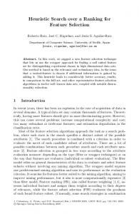
where φ is the angle between the ball direction of travel and the robot, as depicted in Figure 1. Substituting in the righthand sides of equations 1 and 2 into 3 we get: 2 [Vball · t]2 = Dball,bot + [Vbot · t]2 − 2 · Dball,bot · Vball · t · cos(φ)
after rearranging and simplifying we get: 2 2 2 [Vbot − Vball ] · t2 + 2 · Dball,bot · Vball · cos(φ) · t − Dball,bot =0 ∗ More generally we will define D(p, p� ) = �p − p� � l2 as the Euclidean distance between points p and p� .
D_ball
P_ball
P_intercept
I
D_bot
D_ball_bot
Fig. 1.
Letting
P_bot
An illustrative example for calculating the intercept point.
2 2 − Vball a = Vbot b = 2 · Dball,bot · Vball · cos(φ) 2 c = −Dball,bot
Now we can easily solve for t as: √ −b ± b2 − 4ac t= 2a The minimum intercept time is then given by tmin = min(t ∈ R+ ) t
(4)
(5)
That is, the smallest positive real solution of equation 4. If Vbot = Vball then a = 0 and equation 4 no longer applies and the solution is obtained by solving t = −c b . Using the intercept calculation algorithm to obtain tmin , we can now easily solve for the point of interception, pmin , by using equation 1. B. Defensive Position Analysis Using the previously derived algorithm for ball interception we can now analyze a particular defensive position. Consider the one-on-one scenario with one attacker and one defender. Given a position within the defender’s half of the field we would like to find the portion(s) of the goal line which are defendable from position p given the current position of the ball. To do so we create a defensive triangle depicted in Figure 2, whereby the vertices coincide with the ball location and the two extreme end points of the goal line. Case 1: If p lies on the exterior of the defensive triangle, then we calculate the interception time for each extreme point, p1 , p2 , of the goal line. If both points can be defended (i.e., i) tmin < tgoal = D(ball,p , i = {1, 2}) return the whole goal Vball line as defendable. If both points are undefendable, then return an empty set of defendable line segments. In the case one extreme point is defendable while the other is not, we split the line segment into two equal halves and recursively call the same procedure again until we find the defendable and undefendable segments (to within a pre-specified tolerance). This simple algorithm is loosely based on the bisection method for root finding ([8], page 353). For all experiments we set � = 1cm as the tolerance. If a segment length is less than �, implying the ”inflection” point is found to within a distance of 1cm, we simply split the interval in half and return one part as defendable and the other as undefendable. This effectively terminates the recursion process. To calculate the number of times a segment is split before a solution is returned we can set �0 = 340cm, as the length of the goal line, and derive the maximum number of iterations, n, needed to find the
565
set of local searches for each robot. Optimizing each local search then results in globally favorable positioning of each team member. C. Defensive Formation
Fig. 2. Left: Formation of a defensive triangle (in black) with vertices given by ball location and goal line end points. Right: Default Scan lines formed by perpendicular bisectors, {ha , hb , hc } on the left, and by median bisectors, {ma , mb , mc } on the right. For an equilateral triangle hi = mi , but the equality can only happen at a single ball location on the field.
defendable and undefendable segments as: n = �log2 ��0 � = �log2 340 1 � = 9. Since each recursive call, in turn calls the intercept calculation function twice (i.e., once for each end point) the total number of function calls is 18, with each call taking a constant amount of time. Case 2: If p lies in the interior of the defensive triangle, then we split the goal line into two segments. First we create a line L∗ passing through Pball and Pbot . Next we find the point p∗ , where the goal line and the ball/bot line L∗ intersect. Notice that p∗ is a defendable point since the ball cannot be shot through the robot. Hence, by splitting the goal line into two segments at p∗ we can calculate the defendable and undefendable goal segments by calling the procedure from case 1. In this case at most 2 · 9 recursive calls will be made. Thus, to find defendable and undefendable line segments, a bisection search technique is used to recursively split the goal segment into subsegments and invoke the calcIntercept function on the endpoints of each line segment. Position p for a single robot is therefore evaluated on the basis of the resulting length of the defending line segment. In other words, the length of the defendable line segment is the utility value for position p and the defensive position analysis algorithm is the state evaluation function. By searching through defensive positions and maximizing the length of the defendable line segments, a robot can find (near) optimal defensive positions. In turn, this procedure can be applied to each of the defending robots, producing a set of defendable and undefendable line segments for each robot. Finding the line segments undefendable by all robots is then a relatively straightforward procedure of interval merging. By looking at the complement of the union of defendable line segments we can produce a set of globally undefendable line segments. Notice that, this procedure is highly generalizable and applicable for use with any number of players. Furthermore, it is efficient and highly amenable to parallelization. In addition, note that different players (on the same team) can be assigned different line segments to defend and hence different roles. Certainly the goalie should be assigned the goal creese as its defensive line segment. However, the defence robots can be assigned other strategic line segments (e.g., the left flank) within the field in order to help the goalie be more effective. In essence, this approach factorizes the search space into a
To derive an algorithm for defensive formation, consider again the defensive triangle made by the location of the ball and the two extreme points on the goal line segment as depicted in Figure 2. For the one-on-one task, the aim of the single defender is to protect the whole goal line, and hence it is advantageous to be within the aforementioned triangle. Clearly, placing the defender outside this triangular area gives the attacker an advantage, whereby the shooting location can be easily determined to be the farthest point away from the defender. On the other hand, as in the real game of soccer, forcing the goalie to be (roughly) equidistant from the extreme points of the goal posts is advantageous. In turn, the position of the goalie should also be influenced by the position of the ball and the ability of the goalie to intercept the incoming shots on goal (i.e., the velocity of the ball and robot, in our case). Analogously, placing the defender within the interior of the aforementioned triangle is a prerequisite for an effective defence. Unfortunately there are (infinitely) many points within the defensive triangle that a defending robot can occupy. To select a finite number of discrete points within the triangle we first choose a number of line segments within the triangle. By scanning along each line segment (from now on referred to as Scan Line), we can evaluate the quality of each point on the Scan Line by using the defensive analysis algorithm described in the previous section. To make the process tractable, we select a fixed number of points on each scan line to evaluate. 1) Default Scan Lines: used by our defence are depicted in the right illustration of Figure 2. These scan lines correspond to (a) perpendicular bisectors and (b) median bisectors (see caption of Figure 2). As the name suggests, these default scan lines are used in the absence of pertinent information that can be used to bias the search for good defensive positions. Taken as a whole, the bisectors provide a satisficing† solution for searching the triangle interior. Examples of the points searched within the defensive triangle, along the default scan lines are presented in Figure 3. Each point is analyzed using the procedure described in the previous section, and the point with the longest defendable line segment is selected. 2) Bias Scan Lines: are used in place of default scan lines to focus the search on highly desirable positions within the defensive triangle. These bias scan lines are formed by examining the orientation of the attacking robot(s). Consider the situation where the defender cannot cover the whole goal line (for instance due to high velocity of the ball). In this scenario, the robot must select a portion of the goal line to defend. In order to rank goal line intervals, the most † A concept due to Herbert Simon whereby the decision making process chooses an option that, while perhaps not the best, is nevertheless good enough.
566
Additionally, bias lines can be weighted according to the proximity of the corresponding attacker to the defensive line assigned to a particular robot. This would allow the defender to rank the levels of danger, presented by each opponent, to their defensive line and allow the robot to take an appropriate action. D. Summary of Heuristic Search Defence Fig. 3. Default scan lines and the actual points (in red) evaluated along the perpendicular and median bisectors. Notice that the shape of the triangle is determined by the location of the ball, which in turn influences the actual points examined during the search.
Each state within the search space corresponds to a plausible position p on the field. Each state is evaluated using a heuristic guidance function based on the length of the defendable line segment. To make the search tractable we select a discrete number of positions along a discrete number of scan lines, thus pruning the search space to a manageable size. In passing we note that, the more points searched the closer to optimal is the resulting solution. In turn, the more scan lines used and/or the finer the discretization of each scan line, the more points will be produced. As a result, the proposed technique easily scales with increased computational resources. E. Simple Offence
Fig. 4. Bias scan lines and the actual points (in red) evaluated along the bisector. Left: Corresponds to a scenario where the ball is not collinear with the attacker robot and its orientation. Notice that the defender is positioned as if to intercept the ball kicked from the current position of the ball along the current orientation of the attacker. Right: The ball has moved into a collinear position and can be kicked by the attacker. However, since the defender was following the trajectory of the ball and positioned itself along the bias scan line, it is in a position to intercept the kick planned by the attacker.
obvious choice is to examine plausible shooting directions for the opponent robot(s). Intuitively, the most immediate threat arises when the current direction the attacking robot is facing intersects the goal line. However, this intuition is only valid when the attacker is in the possession of the ball. Thus to generalize the notion of immediate threats we project a ray originating at the current location of the ball along the direction of the attacking robot. If this ray intersects the goal line then a new scan line is formed. The bias scan line corresponds to the bisector of the defensive triangle along the aforementioned ray which intersects the goal line. An example of this defensive strategy is presented in Figure 4. As the ball travels towards the attacker, the shape of the defensive triangle is changing and the position of the bias scan line is also changing. By searching through a limited set of positions along the bias scan line the defender can pick the location maximizing the length of the defendable segment along the goal line. When the ball reaches the attacker the defender is in an advantageous position to intercept a kick in the direction faced by the attacker. Although we have proposed several approaches to define the scan lines, our method will search through any set of scan lines and can evaluate an arbitrary number of points along each scan line. Furthermore, the bias scan lines are readily applicable to the real game of RoboCup. Using this anticipatory defense mechanism a goalie can strategically position itself so as to prevent one-timers and breakaways.
Examining the Defensive Position Analysis algorithm presented in section III-B we can immediately see that the exact same approach can be used to deduce the weaknesses within the opponents’ defense. Clearly, knowing which line segments of the goal line are defendable and undefendable gives, in this case, the attacker a tremendous advantage. Consider the one-on-one task, where the attacker has only the choice of the shooting angle to consider (since dribbling is prohibited). Although a relatively easy-to-implement approach for the one-on-one scenario is to simply shoot at a point on the goal line farthest from the robot, this is in fact only correct in restricted situations (such as when the defender is constrained to travelling along the goal line). However, if the defender is close to the center line, a more effective strategy may be to shoot at the point on the goal line orthogonal to the current position of the ball so that the defender has the least amount of time to react. In general, one needs to determine the points on the goal line which are and are not defendable in order to make an intelligent decision. This ‘line’ of thought (no pun intended), in fact, motivates the use of the defensive position analysis algorithm for obtaining a shooting solution. For offense we search over a set of discrete shooting angles. Using the previously described defensive analysis evaluation we calculate the length of the defendable line segments for a given shooting angle. This time however, the search aims to minimize the length of line segments defendable by the opposing team. F. Passer-Receiver Coordination Step 1: Select the robot closest to the ball as the passer and attempt to intercept the ball. The other robot becomes the receiver (in the two-on-two scenario). Clearly, in dynamic real-time environments, such as Robocup, the faster one can get to the ball and start the passing-shooting sequence the less time an opponent has to react.
567
Step 2: Randomly generate a set of plausible receiving locations within a pre-specified radius around the receiving robot. Step 3: Remove infeasible passing locations. For each passing location we use calcIntercept to determine if the receiver can intercept the pass. Step 4: Prune the state space (i.e., the number of feasible positions) based on the following two heuristics: (a) D(p, p� ) < t1 indicating the two feasible points are too close to each other, and (b) D(p, proj(p, LC )) > t2 , where Lc is the center line. This heuristic indicates the distance of point p to the centerline. The closer the robot is to the center line the less time opponent robots have to react to an oncoming shot. Hence, shooting near the centerline makes covering the goal line more difficult for the opponent robots. Step 5: Evaluate the merit of each remaining feasible point. Given a ball location and the location of opponent robots, the value function (which again uses calcIntercept) returns the best shooting direction along with the cumulative intercept times for the opponent robots as a value of the feasible pass location. The value function can also indicate when neither of the opponent robots can intercept the ball before it reaches their goal line, in which case, the receiver automatically shoots instead of passing. Otherwise, a heuristic search over all feasible receiving positions is conducted. The search iteratively examines the likelihood of scoring from each of the proposed receiving positions given the current placements of the opponents. Greedily, the location with the highest score is selected to be the next receiving position. Once a shooting action is selected it cannot be changed back into a passing action. However, at every time-step (while the pass is being executed), the shooting direction is re-evaluated and adjusted based on current placement of the opposing robots. In turn, this calculation is performed using the simple offense routine, which again utilizes the calcIntercept function.
TABLE I R ESULTS FOR O NE - ON -O NE ( TOP ) AND T WO - ON -T WO T OURNAMENTS ( BOTTOM ) BALL SPEED IS DENOTED BY vball . T OTAL SCORES REFLECT THE SUM OF GOALS SCORED OVER THE THREE ROUNDS , WHILE MEAN INDICATES THE NUMBER OF GOALS SCORED BY EACH OPPONENT AVERAGED OVER THE THREE ROUNDS .
One-on-One BSL vs LD BSL vs LD DSL vs LD DSL vs LD DSL vs BSL DSL vs BSL
v_ball 150 250 150 250 150 250
1 5:0 44:30 0:0 37:38 1:1 35:41
Round 2 9:0 46:25 0:0 39:40 1:0 33:41
3 10:0 36:24 3:3 39:39 1:0 35:42
Total 24:0 126:79 3:3 115:117 3:1 103:124
Mean 8.0:0.0 42.0:26.3 1.0:1.0 38.3:39.0 1.0:0.3 34.3:41.6
Two-on-Two PRF vs BSL PRF vs BSL PRF vs DSL PRF vs DSL DSL vs BSL DSL vs BSL
v_ball 150 250 150 250 150 250
1 0:0 0:5 0:0 0:8 0:0 11:16
2 0:0 2:4 0:1 0:7 0:3 10:16
3 0:0 1:11 0:0 1:9 0:4 5:18
Total 0:0 3:20 0:1 1:126 0:7 22:50
Mean 0.0:0.0 1.0:6.7 0.0:0.3 0.3:8.0 0.0:2.3 7.3:16.7
the same simple offense strategy described in section III-E. To evaluate the merits of each approach a small tournament was set up. Each agent played the other agent over three, five minute, rounds in each game. Two sets of experiments were conducted, one using ball speed of 150cm/s and the other using ball speed of 250cm/s. In all experiments the speed of the robots was set at a constant 100cm/s. The results are presented in Table I. Clearly the BSL agent performs much better than the other two agents at higher ball speed and is as good or better at the slow ball speed. Compared to the reactive LD agent our search based BSL approach was able to anticipate shots on goal and effectively intercept every single shot at slow speed. B. Two-on-Two Tournament
IV. E XPERIMENTAL R ESULTS A. One-on-One Tournament To evaluate the merits of basic defensive formation strategies three different agents were created. Bias Scan Line (BSL): agent used bias scan lines to determine its defensive position as described in section III-C. When no immediate threats were detected the agent defaulted to analyzing defensive points along the default scan lines. Default Scan Line (DSL): agent used only points lying on default scan lines for defense. Line Defense (LD): agent was restricted to moving along the goal line (during defensive maneuvers) and focused on shadowing the ball trajectory as it moved from one extreme of the Y-axis to the other. Unlike the first two agents, which are able to plan ahead and anticipate shoots on goal, this is a purely reactive agent. It does not plan ahead but simply reacts to the current position of the ball and was created as a baseline method to test our heuristic search algorithms against. To fairly assess the defensive capabilities of each agent, all agents employed the same ball interception strategy and
This task also used the BSL and DSL agents, whose behavior was the same as in the previous experiment. However, for this experiment the goal line was divided into two (nonoverlapping) segments with each team member defending one of the goal segments. The third agent was designed using the Passer-Receiver Framework (PRF) described in section III-F. In contrast to the other two agents, it had limited defensive capabilities but was able to plan ahead two moves and pass the ball to lucrative locations deemed to be good scoring positions by the evaluation function based on the defensive position analysis algorithm described in section III-B. The agents were evaluated using the same tournament settings as in the previous experiment. In all cases the passing ball speed was set to 100cm/s, to match speed of the robots. Results, presented at the bottom half of Table I, once again indicate that the BSL agent performs much better than the other two agents at higher ball speeds and is as good or better at the slow ball speed.
568
TABLE II PASS C OMPLETION E XPERIMENT Round First Half Second Half
vball = 120 36/37 34/35
vball = 200 47/51 49/53
vball = 250 51/58 50/59
C. Pass Completion To determine how proficient the PRF based offensive strategy is at coordinating passes, a pass completion experiment was conducted. Three experiments were run using passing speeds of 120cm/s, 200cm/s, and 250cm/s. The shooting speed was set at 200cm/s for all experiments. The PRF agent played against the BSL agent but only the number of completed and uncompleted passed was recorded. For each setting two runs, each two minutes in length, were performed. The results are shown in Table II. Each cell represents the number of completed passes total number of passes . We should also point out, that for this and only this experiment we manually set Vball parameter within the PRF to coincide with the actual vball setting in the simulator. The aim of this experiment was to demonstrate that given correct speed estimates, the PRF agent can indeed produce adequate passing behavior in the presence of adversaries (in this case the BSL agent). The results of the pass completion experiments show that in general at lower passing speeds (i.e. 120, 200) the majority of passes are completed successfully. This suggests that the calculation of feasible positions using our conservative reachability computation formula closely estimates the ability of the receiver to intercept the pass. When the passing speed is set to 250, higher number of passes are missed by the receiver. Currently, we believe that this drop in performance is mostly due to the reachability computation not accounting for robot rotation speeds. V. D ISCUSSIONS AND C ONCLUSIONS Having analyzed the individual performance of our defensive (BSL, DSL) and offensive strategies (PRF and simple offence) future research will examine the performance of an integrated BSL+PRF agent. The fact that BSL did not lose a single game in both one-on-one and two-on-two competition demonstrates the effectiveness of anticipatory defensive strategies. The effectiveness of the PRF framework was established by experiment three demonstrating the high number of completed passes. An interesting future research direction would be attempting to combine machine learning methods together with heuristic search methods. The time spent on this research project was heavily biased towards low level development of primitive actions such as moving to the ball at a correct angle for a kick or a pass, or coordinating the receiver’s orientation. A search akin to the one presented in this paper, could be conducted over the high-level machine-learned behaviors rather than the low-level actions.
On a more general note, we would like to point out once again that the algorithms developed in this paper are easily extendable and applicable to the real game of RoboCup and can indeed be beneficial for both defensive and offensive strategies. By converting a 2D coordination problem into a set of local searches, which reason about line segments, we have greatly simplified the problem. Each local search optimizes the behavior of a single robot. Observe we have eliminated the need for opponent modeling by reasoning about worst case scenarios. In essence our framework tries to answer two simple questions (a) In the case of defense can we defend our line segment? (b) In the case of offence can the opponent defend its line segment? Since line segments can be placed anywhere on the field we can reason about passing, shooting, and interception strategies as well as defensive formations with a single unified framework. In summary, this paper focused on developing heuristic search-based algorithms for real-time continuous action adversarial environments. The classic search algorithms designed for games like chess, the depth of the search is the key determinant of solution quality. Such approaches are completely infeasible since actions are not deterministic, moves can be simultaneous, and the branching factor is immense. In contrast, the proposed approach aims to identify key skills needed for a robot to be competent within a given domain. In turn, each skill can be effectively reused and translated into an accurate heuristic guidance function allowing the search to be wide but shallow. As demonstrated by the experimental results, the proposed approach can be effective in coordinating agents within adversarial environments. R EFERENCES [1] Michael Bowling and Manuela Veloso. Simultaneous adversarial multirobot learning. In Proceedings of International Joint Conference on Artificial Intelligence, 2003. [2] Peter E. Hart, Nils J. Nilsson, and Bertram Raphael. A formal basis for the heuristic determination of minimum cost paths. SIGART Bull., (37):28–29, 1972. [3] D. E. Knuth and R. W. Moore. An analysis of alpha-beta pruning. Artificial Intelligence, 6(4):293–326, 1975. [4] Richard E. Korf. Depth-first iterative-deepening: an optimal admissible tree search. Artif. Intell., 27(1):97–109, 1985. [5] Richard E. Korf. Real-time heuristic search. Artificial Intelligence, 42(23):189–211, 1990. [6] James J. Kuffner and Steven M. LaValle. RRT-connect: An effcient approach to single-query path planning. In Proceedings of IEEE International Conference on Robotics and Automation, 2000. [7] Matthew McNaughton, Sean Verret, Andrzej Zadorozny, and Hong Zhang. Broker: An interprocess communication solution for multi-robot systems. In Proceedings of International Conference on Intelligent Robots and Systems, 2005. [8] W.H. Press, S.A. Teukolsky, W.T. Vetterling, and B.P. Flannery. Numerical Recipes in C: The Art of Scientifi Computing, Second Edition. Cambridge University Press, 2002.
569