Hierarchical Bayesian regularization of reconstructions for diffuse optical tomography using multiple priors Farras Abdelnour,1 Christopher Genovese,2 and Theodore Huppert1,3* 1 Department of Radiology, University of Pittsburgh, 200 Lothrop St. Pittsburgh PA 15213, USA Department of Statistics, Carnegie Mellon University, 5000 Forbes Ave. Pittsburgh PA 15213, USA 3 Department of Bioengineering University of Pittsburgh, 300 Technology Dr. Pittsburgh PA 15219, USA *
[email protected] 2
Abstract: Diffuse optical tomography (DOT) is a non-invasive brain imaging technique that uses low-levels of near-infrared light to measure optical absorption changes due to regional blood flow and blood oxygen saturation in the brain. By arranging light sources and detectors in a grid over the surface of the scalp, DOT studies attempt to spatially localize changes in oxy- and deoxy-hemoglobin in the brain that result from evoked brain activity during functional experiments. However, the reconstruction of accurate spatial images of hemoglobin changes from DOT data is an illposed linearized inverse problem, which requires model regularization to yield appropriate solutions. In this work, we describe and demonstrate the application of a parametric restricted maximum likelihood method (ReML) to incorporate multiple statistical priors into the recovery of optical images. This work is based on similar methods that have been applied to the inverse problem for magnetoencephalography (MEG). Herein, we discuss the adaptation of this model to DOT and demonstrate that this approach provides a means to objectively incorporate reconstruction constraints and demonstrate this approach through a series of simulated numerical examples. ©2010 Optical Society of America OCIS codes: (170.3010) Image reconstruction techniques; (170.2655) Functional monitoring and imaging.
References and links 1. 2. 3. 4. 5. 6. 7.
8. 9.
D. A. Boas, A. M. Dale, and M. A. Franceschini, ―Diffuse optical imaging of brain activation: approaches to optimizing image sensitivity, resolution, and accuracy,‖ Neuroimage 23(Suppl 1), S275–S288 (2004). T. J. Huppert, M. S. Allen, S. G. Diamond, and D. A. Boas, ―Estimating cerebral oxygen metabolism from fMRI with a dynamic multicompartment Windkessel model,‖ Hum. Brain Mapp. 30(5), 1548–1567 (2009) (PMCID: 2670946.). T. Wilcox, H. Bortfeld, R. Woods, E. Wruck, and D. A. Boas, ―Using near-infrared spectroscopy to assess neural activation during object processing in infants,‖ J. Biomed. Opt. 10(1), 011010 (2005). S. Perrey, ―Non-invasive NIR spectroscopy of human brain function during exercise,‖ Methods 45(4), 289–299 (2008). I. Miyai, H. C. Tanabe, I. Sase, H. Eda, I. Oda, I. Konishi, Y. Tsunazawa, T. Suzuki, T. Yanagida, and K. Kubota, ―Cortical mapping of gait in humans: a near-infrared spectroscopic topography study,‖ Neuroimage 14(5), 1186–1192 (2001). U. Sunar, S. Makonnen, C. Zhou, T. Durduran, G. Yu, H. W. Wang, W. M. Lee, and A. G. Yodh, ―Hemodynamic responses to antivascular therapy and ionizing radiation assessed by diffuse optical spectroscopies,‖ Opt. Express 15(23), 15507–15516 (2007). U. Sunar, H. Quon, T. Durduran, J. Zhang, J. Du, C. Zhou, G. Yu, R. Choe, A. Kilger, R. Lustig, L. Loevner, S. Nioka, B. Chance, and A. G. Yodh, ―Noninvasive diffuse optical measurement of blood flow and blood oxygenation for monitoring radiation therapy in patients with head and neck tumors: a pilot study,‖ J. Biomed. Opt. 11(6), 064021 (2006). S. R. Arridge, ―Optical tomography in medical imaging,‖ Inverse Probl. 15(2), 14–93 (1999). A. P. Gibson, J. C. Hebden, and S. R. Arridge, ―Recent advances in diffuse optical imaging,‖ Phys. Med. Biol. 50(4), R1–R43 (2005).
#133504 - $15.00 USD
Received 19 Aug 2010; revised 2 Oct 2010; accepted 2 Oct 2010; published 6 Oct 2010
(C) 2010 OSA
1 November 2010 / Vol. 1, No. 4 / BIOMEDICAL OPTICS EXPRESS 1084
10. J. Mattout, C. Phillips, W. D. Penny, M. D. Rugg, and K. J. Friston, ―MEG source localization under multiple constraints: an extended Bayesian framework,‖ Neuroimage 30(3), 753–767 (2006). 11. K. J. Friston, Statistical parametric mapping: the analysis of functional brain images. 2007, London: Academic. vii, 647. 12. R. W. Cox, ―AFNI: software for analysis and visualization of functional magnetic resonance neuroimages,‖ Comput. Biomed. Res. 29(3), 162–173 (1996). 13. A. Li, Q. Zhang, J. P. Culver, E. L. Miller, and D. A. Boas, ―Reconstructing chromosphere concentration images directly by continuous-wave diffuse optical tomography,‖ Opt. Lett. 29(3), 256–258 (2004). 14. D. Harville, ―Maximum likelihood approaches to variance component estimation and related problems,‖ J. Am. Stat. Assoc. 72(358), 320–338 (1977). 15. K. J. Friston, W. Penny, C. Phillips, S. Kiebel, G. Hinton, and J. Ashburner, ―Classical and Bayesian inference in neuroimaging: theory,‖ Neuroimage 16(2), 465–483 (2002). 16. K. J. Friston, D. E. Glaser, R. N. Henson, S. Kiebel, C. Phillips, and J. Ashburner, ―Classical and Bayesian inference in neuroimaging: applications,‖ Neuroimage 16(2), 484–512 (2002). 17. A. P. Dempster, N. M. Laird, and D. B. Rubin, ―Maximum likelihood from incomplete data via the EM algorithm,‖ J. R. Stat. Soc., B 39(1), 1–38 (1977). 18. D. K. Joseph, T. J. Huppert, M. A. Franceschini, and D. A. Boas, ―Diffuse optical tomography system to image brain activation with improved spatial resolution and validation with functional magnetic resonance imaging,‖ Appl. Opt. 45(31), 8142–8151 (2006). 19. F. Abdelnour, B. Schmidt, and T. J. Huppert, ―Topographic localization of brain activation in diffuse optical imaging using spherical wavelets,‖ Phys. Med. Biol. 54(20), 6383–6413 (2009) (PMCID: 2806654.). 20. I. Daubechies, Ten Lectures On Wavelets. SIAM, 1992. 21. T. J. Huppert, S. G. Diamond, and D. A. Boas, ―Direct estimation of evoked hemoglobin changes by multimodality fusion imaging,‖ J. Biomed. Opt. 13(5), 054031 (2008). 22. D. A. Boas, and A. M. Dale, ―Simulation study of magnetic resonance imaging-guided cortically constrained diffuse optical tomography of human brain function,‖ Appl. Opt. 44(10), 1957–1968 (2005). 23. B. W. Pogue, S. C. Davis, X. Song, B. A. Brooksby, H. Dehghani, and K. D. Paulsen, ―Image analysis methods for diffuse optical tomography,‖ J. Biomed. Opt. 11(3), 033001 (2006).
1. Introduction Diffuse optical tomography (DOT) is a non-invasive technology which uses low-levels of non-ionizing light in the range of 650-900nm to record changes in the optical absorption and scattering of tissue. Over the past thirty years, the use of DOT for non-invasively imaging the human brain has been steadily growing as reviewed in [1]. As compared with functional MRI (fMRI), DOT is less costly, more portable, and allows for a wider range of experimental scenarios because it does not require a dedicated scanner nor require the subject to lay supine. Moreover, optical imaging has the ability to resolve changes in both oxy- and deoxyhemoglobin (denoted HbO2 and Hb respectively) within the brain using multiple wavelengths of light, which can potentially lead to the ability to discriminate blood flow and oxygen metabolism changes [2]. Examples of niche applications for optical brain research have included studies on infant and child brain activation [3], studies of activation during exercise and mobility [4,5], bedside monitoring of clinical patients [6,7], as well as more traditional cognitive testing and psychology studies. Because of its low cost of operation and portability, DOT has been growing in popularity in these fields over the last several years. Although a strength of optical imaging is its temporal resolution (several hertz) and ability to detect both oxy- and deoxy-hemoglobin, optical imaging can also provide some degree of specificity to spatially localize regions of brain activity through the reconstruction of images from data collected via multiple optical light emitter and detector pairs. In a typical optical brain imaging experiment, a grid of light emitters and detectors is placed on the surface of the scalp as shown in Fig. 1. The optical absorption changes recorded from light diffusely traveling between emitter and detector pairs can be used to recover low-resolution spatial images of the underlying blood flow changes. However, such images are often difficult to accurately recover due to optical scattering in the tissue, the limited number of measurements typically available, and the inverse problem of estimating changes within the underlying volume of tissue (brain) from measurements made only on the surface of the head. The estimation of optical images is generally both under-determined (more unknowns than measurements) and ill-posed (no single unique solution). The optical inverse problem has been reviewed in [8].
#133504 - $15.00 USD
Received 19 Aug 2010; revised 2 Oct 2010; accepted 2 Oct 2010; published 6 Oct 2010
(C) 2010 OSA
1 November 2010 / Vol. 1, No. 4 / BIOMEDICAL OPTICS EXPRESS 1085
Fig. 1. Diffuse optical imaging uses fiber optic based light sources and detectors to record changes in the optical absorption of underlying tissue. A grid of sensors is placed noninvasively on the head of a participant and used to measure changes in oxy- and deoxyhemoglobin in the brain during task-evoked activation. The source-detector arrangement in the probe above is shown in Fig. 2.
Active research on the optical inverse problem has lead to continued improvements in recent years and for an overview of image reconstruction techniques see [9]. To date, much of the work on the optical inverse problem has involved the use of regularization priors, such as the weighted minimum norm (WMN) or Tikhonov regularization. In general, regularization methods require an estimate of weight (trust) given to the regularization penalty (prior) that is usually predefined or manually tuned to yield acceptable images. One of the difficulties of these techniques, therefore, is the need for an a priori choice of this weight or weights in the case of multiple priors. In this paper, we will describe how the restricted maximum likelihood (ReML) method and a Bayesian formulation can be used to stabilize the optical inverse problem and introduce multiple statistical priors. ReML has been introduced previously in the field of magnetoencephalography (MEG) for a similar inverse model [10]. This method is also the basis of a deconvolution model currently implemented for the time-series analysis of fMRI data within the software packages SPM (statistical parametric mapping [11]) and AFNI (analysis of functional neuroimages [12]). The purpose of this paper is not to exhaustedly cover the theory behind the ReML method, which can be found in previous literature (see [11] for a review). Instead, we will briefly outline the concept, describe how to implement this method for optical spatial inverse problems, and provide several demonstrations of how this approach can be used to optimally introduce multiple priors into optical reconstructions. Throughout this paper, we will present numerical examples of this model with increasing complexity in order to gradually introduce components of this method. First, in initial demonstrations, we will first show that for the case of a single minimum norm prior model (similar to the widely used Tikhonov regularization to the optical inverse problem), the ReML method produces identical results to those obtained through optimized regularization via the L-curve method. In later sections of this work, we generalize this model to show that the ReML method allows the incorporation of additional priors including assumptions about the physiology of the brain’s response and region-of-interest information. We will finally show how the ReML method can be used to independently tune the Bayesian noise model in the brain and superficial layers to create depth discrimination and to separate superficial noise and brain activity signals. 2. Theory The optical forward model Diffuse optical brain imaging has been described in several recent reviews [1]. In this section, we will only briefly describe the setup and recording of optical data as it pertains to the optical spatial inverse problem. In a typical DOT experiment, a grid of light emitters and detectors is
#133504 - $15.00 USD
Received 19 Aug 2010; revised 2 Oct 2010; accepted 2 Oct 2010; published 6 Oct 2010
(C) 2010 OSA
1 November 2010 / Vol. 1, No. 4 / BIOMEDICAL OPTICS EXPRESS 1086
positioned on the surface of the scalp of the subject (see Fig. 1). At each of these emitter positions, light is sent into the tissue at two or more wavelengths. Due to the highly scattering nature of biological tissue, this light spreads as it enters the tissue. For samples thicker than a few millimeters, the propagation of light through tissue is often approximated by a diffusionbased random walk of the photons of light and can be modeled through Monte Carlo, finite difference, finite element, or boundary element methods. The propagation of the light depends on the structure of the underlying layers of the tissue (in our case; the scalp, skull, cerebral spinal fluid, and gray/white matter layers of the head), which defines the volume sampled by each optical emitter and detector combination. The optical measurement model is approximated by the expression OD i , j L i , j A , S G i , j i , j
(1)
where OD is the measured optical density and is defined as I i, j OD i , j Log I 0 (2) In Eq. (2), I is the intensity of light exiting the tissue and Io is the light entering the tissue. G is a geometry dependent factor. In Eq. (1), υ is an additive noise in the measurement space (e.g. instrument noise), which will be emphasized further in the context of the ReML model. Lijλ is the optical measurement model obtained from estimation of the ensemble path of photons through the tissue and describes the summation of absorption values μA along the diffuse path traveled by the light going from a particular light emitter to a detector pair (i,j). Both μA and μs are vectors of the absorption and scattering values at each position in the volume and can be reshaped as an image of these changes. During brain activity, regional changes in blood flow alter the concentration of hemoglobin in the brain and in turn change the absorption of the tissue. In this work, we will ignore scattering changes associated with brain activity although the model we will describe can be easily extended to deal with scattering as well. For small changes in absorption, as typically observed for brain activity studies, the change in optical density ΔOD is approximated by linearization of Eq. (1) around the baseline values of μA and μs and subtraction of the baseline absorption. OD i , j A i , j A , S A i , j
(3)
ΔμA is a vector of the changes in absorption at each position (voxel) in the underlying tissue. Aijλ is the Jacobian of the optical measurement model. Equation (3), describes the optical forward model describing the change in optical signal caused by changes in the absorption in the underlying tissue for one particular wavelength of light and set of baseline optical properties. Typically in brain imaging studies, two or more wavelengths of light are used to provide an ability to distinguish changes in both oxy-hemoglobin (HbO2) and deoxyhemoglobin (Hb). The overall absorption at each wavelength is a linear combination of the contributions from each chromophore and is given by the Beer-Lambert expression
A , HbO HbO2 HbO2 Hb Hb Hb , 2
(4)
where ελHbX is the molar extinction coefficient for oxy- or deoxy-hemoglobin at the particular wavelength and describes the wavelength specific absorption properties of these chromophores per molar unit of concentration. ωHbX is a second type of additive noise (or uncertainty error) term acting in the image (brain) space and is distinct from the measurement space noise (υ). We will clarify this distinction later in the context of the ReML model. Again, ΔμA, Δ[HbX], and ω are vectors representing these changes at each position in the tissue. Equation (4) can be substituted into the optical forward model to produce the optical measurement model with spectral priors (e.g. Li et al [13]) #133504 - $15.00 USD
Received 19 Aug 2010; revised 2 Oct 2010; accepted 2 Oct 2010; published 6 Oct 2010
(C) 2010 OSA
1 November 2010 / Vol. 1, No. 4 / BIOMEDICAL OPTICS EXPRESS 1087
OD i , j A i , j HbO HbO2 HbO2 Hb Hb Hb i , j 2
(5)
From here on, the dependence of the forward model (Ai,j) on baseline absorption and scattering coefficients will be no longer explicitly written (e.g. Aλi,j = Aλi,j(μλA, μλS’) ). Changes in oxy- and deoxy-hemoglobin can be inferred from optical measurements at multiple (N) wavelengths by means of solving a set of linear equations given by
1 1 1 OD i , j A i , j HbO2 OD 2 2 2 i, j A i , j HbO2 N OD i , j A N N i, j HbO2
1 (6) 1 HbO A i , j Hb HbO2 i , j 2 2 2 Hb A i , j Hb Hb i , j N N i , j A i , j Hb
and λi denotes the ith-wavelength. Hereafter, the optical forward model will be written in the more compact form Y H
(7)
where the new variable β has been introduced to describe the unknown values of the combination of oxy- and deoxy-hemoglobin changes in the tissue, given by
(8) HbO2 Hb In summary, Eqs. (7) and (8) describe the linear relationship between changes in concentrations of HbO2 and Hb in the tissue, and the changes in optical density as recorded on the surface between optical sources and detectors. It is this equation that must be inverted in order to reconstruct an image (volume) of the hemodynamic changes in the brain. The optical inverse problem The estimation of optical images by the inversion of Eq. (7) entails an underdetermined problem where there generally are significantly less available measurements (Y) than unknown parameters (β) in the image to-be-estimated. This means that, in general, there is not enough information in the measurements alone to yield accurate and unique estimates of images of brain activity. There are two general approaches to solving this problem— regularization and Bayesian theories. In general, regularization theory (including Tikhonov regularization) has been most widely used and is more familiar to practitioners of the optical inverse problem. On the other hand, ReML and our current work are based on the Bayesian interpretation. For this reason, we will briefly attempt to reconcile these two theories noting that for a subset of regularization models in the class of linear-quadratic regularization (which includes many of the current optical inverse models), there is an equivalent Bayesian interpretation of the model. Regularization methods attempt to stabilize the solution of the inverse problem by extending the objective function used to minimize the problem by adding additional penalty terms. For example, in conventional least squares inverse models, the least-squares cost function minimizes the mean squared error of the model to fit the data. In the case of the linear model Y = H·β, the least squares solution is given by arg min
Y H
2
(9)
N
In other words, Eq. (9) aims to find the value of the parameter set (β) that minimizes the error
to
the
measured
data.
The
notation
X
2 N
denotes
the
weighted
norm
#133504 - $15.00 USD
Received 19 Aug 2010; revised 2 Oct 2010; accepted 2 Oct 2010; published 6 Oct 2010
(C) 2010 OSA
1 November 2010 / Vol. 1, No. 4 / BIOMEDICAL OPTICS EXPRESS 1088
( X N X T N X ). Generalized Tikhonov regularization extends this least-squares cost function by adding a penalty for deviations of β from some prior expected value of the parameter (β0) and is given by the minimization expression 2
Y H
arg min
2 N
0
2
(10)
P
The term λ is a hyper-parameter, which is used to tune the model. In the case that λ is small, the solution favors minimizing the residual error with the measured data and likewise when λ is large, the solution is biased towards matching the prior (β0). A typical assumption in the optical inverse model is that β0 is zero, which results in what is called the minimum norm solution. The regularization model can be extended to add additional penalty terms. For example, Li et al [13] extended this model with a second penalty term which applied only to parameters outside of a predefined region-of-interest (for example regions selected from MRI segmentation). The cost function proposed by Li et al was: arg min
Y H
2 I
1 M
2 I
2 1 M
2 I
(11)
where M specifies a binary mask of a predefined region-of-interest such that M
1 if in region-of-interest
(12)
0 else The Li et al model thus had two regularization hyperparameters (λ1 and λ2), which applied penalties to the parameters inside and outside of the region-of-interest respectively. Alternative regularization models have been proposed to add low-pass or high-pass operators to impose smoothness on the solution. In regularization models, the L-curve technique and generalized cross-validation can be used to optimally select the hyperparameters of the model. However to date, many optical reconstruction methods have used λ as a manual tuning parameter allowing images to be adjusted in a subjective optimization. In general terms, the regularization hyperparameter (λ) is a weight that is assigned to that penalty term in the cost function. Linear quadratic regularization models are a subset of regularization cost functions that only contain L2 norm penalty terms such as those described in Eqs. (9)–(11). The cost function can be viewed as a weighted penalization for the distance of the solution from the priors (either the measurement itself or the prior on the solution; e.g. β0). In the regularization model, these distance penalties (e.g. N and λ·P in Eq. (10) can be somewhat arbitrary provided that they are symmetric matrices. In contrast, the Bayesian model offers an alternative interpretation by suggesting that the optimal distance weight should be the inverse of a covariance matrix. For example, in Eq. (10), the weighted norm penalty N should be the inverse of the measurement noise covariance and from the second term, the value of λ·P should be the inverse of the parameter covariance. In terms of the optical inverse model, these two terms are the covariance of υ and ω respectively from Eq. (7). Whether one interprets Eq. (10) from a (linear-quadratic) regularization or Bayesian prospective, the solution to the linear model (Y = H·β) is the same and is given by the GaussMarkov equation:
0 H T N H P H T N Y H 0 1
(13)
In the case of the Bayesian model, N and λ·P would be given by the inverse of the measurement and parameter covariance models (which we will later denote CN and CP following the convention of the SPM software).
#133504 - $15.00 USD
Received 19 Aug 2010; revised 2 Oct 2010; accepted 2 Oct 2010; published 6 Oct 2010
(C) 2010 OSA
1 November 2010 / Vol. 1, No. 4 / BIOMEDICAL OPTICS EXPRESS 1089
Restricted Maximum Likelihood (ReML) While regularization models are not restricted to linear quadratic expressions and are thus more general than Bayesian models, the Bayesian point-of-view offers additional optimization methods to select the hyperparameters of the model (e.g. λ) as alternatives to L-curve or crossvalidation methods. In particular, under the Bayesian point-of-view and the interpretation of N and P as the inverse of covariance matrices, additional objective functions such as the maximum likelihood of the model can be used to optimize the hyperparameters. Restricted maximum likelihood was introduced by Harville [14] as a method to produce unbiased estimates of the covariance parameters of a linear mixed model under Bayesian assumptions. This approach is implemented in several commercial statistical packages such as SPSS in the MIXED function. In the context of neuroimaging ReML was introduced by Friston et al for the stabilization of the temporal deconvolution model used for analysis of brain activity images in functional MRI [15,16]. This is implemented in the software SPM (Statistical Parametric Mapping [11]; ). This method was later implemented in the context of the ill-posed image reconstruction inverse model for magnetoencephalography (MEG) and electroencelography (EEG) also within the SPM software [10]. Details of the derivation and theory behind the ReML model are described in several papers by Friston et al [15,16]. In brief, ReML is based on the maximization of the loglikelihood of the data conditional on the set of hyperparameters (e.g. p(Y|λ)). It can be shown that (see appendix 3 of [11]) maximization of the log-likelihood function is equivalent to maximizing the free-energy of the model and is given by the expression:
1 1 1 1 2 2 (14) Y H C 0 C Log CN Log CP N P 2 2 2 2 ,CN ,CP Note that this is similar to the previous weighted least-squares cost function expression with the addition of log-determinant penalties for the covariance terms and a change in sign of all the terms. Rather than solving for the full covariance matrices (CN and CP) from Eq. (14), the covariance models can be parameterized as a linear combination of covariance components. For example: arg max
CN i QN ,i i
CP j QP , j
(15)
j
where QN and QP are symmetric matrices that can be used to build up the covariance model. In the example of the optical model, CN represents the covariance of the measurement noise and thus, two (or more) diagonal covariance components (QN) might be used with each representing the variance on one of the two (or more) measured optical wavelengths. In the methods section, we will further detail the selection of these components for the optical model. The hyper-parameters (Λ; upper-case lambda) in Eq. (15) adjust the weighting of these covariance components. Again, in the context of the two wavelength optical model, there would be two hyper-parameters allowing adjustment of the noise at the two wavelengths. Note in reference to the work by Friston et al [15] for the derivation of the ReML model, a lower-case lambda (λ) is used and has been switched here for distinction from the term as used in the context of the regularization model. In order to solve the ReML model, the expectation-maximization (EM) algorithm [17] can be used. In order to minimize the parameterized form of Eq. (14) for both the parameters (β) and the hyperparameters (Λ), the EM model alternates between estimation of both types. First given an estimate of the hyperparameters, the Gauss-Markov expression is solved to estimate the parameters:
0 H T C 1N H CP 1 H T C 1N Y H 0 1
(16)
#133504 - $15.00 USD
Received 19 Aug 2010; revised 2 Oct 2010; accepted 2 Oct 2010; published 6 Oct 2010
(C) 2010 OSA
1 November 2010 / Vol. 1, No. 4 / BIOMEDICAL OPTICS EXPRESS 1090
Note, Eqs. (13) and (16) are identical, where we have just substituted to the specific Bayesian form of the model. Once the parameters of the model are estimated from Eq. (16) (expectation step), the Eq. (14) is maximized for the hyperparameters (Λ) in the maximization step. The matrix derivative of Eq. (14) with respect to the vector of hyperparameters is set to zero and solved to yield an updated estimate of these hyperparameters. These are substituted back into Eq. (16) to re-estimate the model parameters. This is repeated until convergence is met. In our model, we defined convergence by the change in the free energy of the model [Eq. (14)], which we describe further in the methods section. 3. Methods In this paper, we will demonstrate the application of a ReML model to the optical inverse problem using several numerical examples. In this section, we will detail the procedure to generate these simulations and the practical implementation of the ReML model as specifically related to our optical model. Calculation of optical forward model In this study, we used a semi-infinite homogeneous slab model for the calculation of the optical forward model. We have chosen to use this model for computational reasons, because this geometry has a known analytic solution, however, this regularization model can be extended for any such forward model. For the simulations, we used an overlapping (tomography) imaging probe as described in Joseph et al [18]. A total of 8 sources and 15 detectors were used with a nearest neighbor distance of 2.5mm and a second nearest neighbor distance of 4.2mm. The probe geometry used in this study is shown in Fig. 2. Measurements were simulated at 830nm and 690nm matching the optical system in our lab.
Fig. 2. Simulation (A) and optical probe geometry (B) used in the construction of sample problems in this work. This probe was based on a tomography (over-lapping measurement) design described in [18] consisting of eight source positions (circles) and fifteen detector postions (squares).
We generated four types of simulated activations. In the first examples of this model, we used a single layered model of size 16x16x1 voxels [6.7mm x 6.7mm x 10mm]. An activation spot (13.4mm x13.4mm) was added in oxy-hemoglobin ( + 1.0μM) and deoxy-hemoglobin (0.25μM). Measurement noise was added to the measurement vector to reach the desired signal-to-noise ratio for each section. In the later set of examples, a more realistic two-layer model was used to mimic the superficial skin and brain layers. Low-frequency additive image-space noise was placed in the superficial layer to mimic systemic noise in some simulations. Finally, in the last examples the reconstruction of multiple loci of brain activity was examined. Wavelet reparameterization of DOT inverse model As noted above, the optical forward model is the product of a non-square sensitivity matrix H and the vector of unknowns β. The matrix H projects the hemoglobin concentration changes from points in the volume of tissue to the expected optical density changes measured at the surface by a particular grid of optical source-detector pairs. In a recent paper [19], we #133504 - $15.00 USD
Received 19 Aug 2010; revised 2 Oct 2010; accepted 2 Oct 2010; published 6 Oct 2010
(C) 2010 OSA
1 November 2010 / Vol. 1, No. 4 / BIOMEDICAL OPTICS EXPRESS 1091
described the use of wavelets as basis set on which to reconstruct optical images. The advantage of the wavelet-based reparameterization of the model is that the specific wavelet filter banks (low-pass, band-pass(es), high-pass) can be biased in the reconstruction as a means of imposing spatial smoothing on the reconstructed image. The wavelet transform can be thought of as a reparameterization of a signal or image in a sense similar to a Fourier transform. However, unlike the Fourier transform, wavelets allow localization in both spatial location and spatial frequency (or time and temporal frequency). By representing the model in the wavelet domain, the different levels of spatial frequencies can be separately regularized through the ReML method. Thus, in the same way that the choice of two Λ’s can be used to adjust the variance (regularization) in the skin and deeper layers, the wavelet model allows us to independently adjust the bias towards or away from a specific spatial frequency band. In the context of diffuse optical image reconstruction, we will show that the wavelet representation offers an ability to distinguish superficial physiology and evoked brain signals on the basis of a priori knowledge that these two signals compose different spatial characteristics. In our work in [19] we described a detailed wavelet model based on the extracted curvature of the cortex. In this current work, we will use a much simpler (conventional) set of wavelets as a means to better demonstrate the current model with less confusion. In our model, we will find β by first reparametrizing the model using orthogonal wavelet transform and then estimating the coefficients βw of the wavelet transform of β. The orthogonal wavelet transformation is a reversible rotation which can be expressed in a matrix notation such that
W W W T W
(17)
where W is the wavelet analysis model (transformation from image to wavelet space). Here, . In this work we use the Daubechies wavelet [20] generated by FIR orthogonal filters of length 2 coefficients and separable in the x-y (in-plane) dimension. Equation (7) is now restated for each layer in terms of wavelets as Y H W T W W
(18) Equation (18) is the optical forward model in the wavelet domain. The parameter noise term (ωW) is now also in the wavelet domain. Since we intend to use a structure to the covariance components, which allows a non-white spatial frequency distribution (particularly to model systemic physiological noise), we will define the covariance components of the ReML model directly in the wavelet domain. The structure of the wavelet matrix W is shown in Fig. 3. The low-pass, band-pass, and high-pass components map to regions of the matrix. Figure 3 shows the structure of this model for the one-dimensional with only 2 stages for simplicity. The actual model used a two-dimensional structure (in the x/y plane) with three stages.
Fig. 3. The optical inverse model was reparameterized in terms of wavelet coefficients. In the wavelet representation, the original image is described as a linear combination of low-pass, band-pass, and high-pass filter banks (left; for 1-dimensional case). The wavelet transform can be implemented in matrix form, which has the same filter structure (right) and will be used to apply a frequency bias to the superficial and deeper layers of the reconstruction.
#133504 - $15.00 USD
Received 19 Aug 2010; revised 2 Oct 2010; accepted 2 Oct 2010; published 6 Oct 2010
(C) 2010 OSA
1 November 2010 / Vol. 1, No. 4 / BIOMEDICAL OPTICS EXPRESS 1092
Example Covariance Components In the parametric Bayesian model, the covariance of the extended measurement vector is described as a weighted linear combination of covariance components, which capture specific a priori features of the model. In this section, we will detail the covariance components that will be discussed in the remainder of this paper. Minimum norm prior. In order to compare against the Tikhonov regularization methods, the minimum norm (covariance) prior should take the form CN = Λ1·I and CP = Λ2·I where both oxy- and oxy-hemoglobin are modeled by a single covariance component and hyperparameter. CN and CP define the total noise model via Eq. (15). This produces the effect of a single hyperparameter to tune the model and is equivalent to the Tikhonov regularization model
H T H I H T Y 1
(19)
where the ratio of Λ1 and Λ2 from the Bayesian model are replaced by the single regularization term λ. Measurement noise prior. In general, optical recordings will have different noise depending on the wavelength. While this is less of a concern for systems with only two measured wavelengths, combining more than two wavelengths into estimates of oxy- and deoxy-hemoglobin via the modified Beer-Lambert law requires an estimate of the noise at each wavelength leading to the weighted least-squares model. In order to model this, CN is modeled by a separate component for each of the measurement types with unity values allow the corresponding diagonal elements for each wavelength type. Thus, the two-wavelength optical model, which we will use in this work, will have two hyper-parameters to define the measurement covariance (CN). While this paper is concerned with optical-only reconstructions, we note that this approach is amendable to multimodal data as well, for example, the joint image reconstruction of brain activity from concurrent optical and functional MRI data as shown in Huppert et al [21]. Separation of HbO2 and Hb. One of the limitations of the Tikhonov approach is that the same level of variance is assumed for the entire parameter space, namely both oxy- and deoxy-hemoglobin. To model different noise levels for both oxy- and deoxy-hemoglobin, the CP component of the covariance matrix can be modeled as a linear combination of two unitydiagonal covariance components corresponding to the two chromophores of the model. We can also impose additional statistical relationships between oxy- and deoxy-hemoglobin, such as the observation that these changes are often anti-correlated (e.g. the typical hemodynamic response involves oxy-hemoglobin increasing and deoxy-hemoglobin decreasing). This can be modeled by negative-signed off-diagonal elements to the covariance components, e.g. (20) QHbO2 / Hb 0 I HbO2 / Hb I 0 HbO2 / Hb Note that this term will be multiplied by a to-be-estimated hyperparameter, which will rescale the covariance. Depth specific spatial frequency priors. As previously discussed, the reparameterization of the optical forward model via the wavelet transform allows statistical priors to impose relationships between the levels of spatial frequency. Namely, the variance of the corresponding low-pass, band-pass, and high-pass wavelet coefficients can be reweighted according to a priori assumptions, such as the expectation that superficial (systemic) signals will be low frequency. By weighting the variance between each frequency band, a covariance component acting as a low-pass filter can be constructed.
#133504 - $15.00 USD
Received 19 Aug 2010; revised 2 Oct 2010; accepted 2 Oct 2010; published 6 Oct 2010
(C) 2010 OSA
1 November 2010 / Vol. 1, No. 4 / BIOMEDICAL OPTICS EXPRESS 1093
(21) QLow pass I Low pass 1 I 2 Band pass 1 I 4 High pass The parameter σ is a smoothing factor. In principal, this term could be included in the list of hyper-parameters and solved, however, this would create a non-linear model and is beyond the current scope of this work. Here, we have used a fixed value of σ = 15mm ( = 2.2 voxel dimensions) in the model. Incorporating prior knowledge of location of ROI. Finally, the covariance components of the ReML model can be used to impose a priori knowledge of regions-of-interest for the location of activation. Such prior information can be obtained for example from experience or from alternate modality such as functional MRI or atlas based priors. The resulting Q’s can then be given by the diagonal matrices for HbO2 and Hb: QROI {i , j}
1 if {i,j} in region-of-interest 0
(22)
else
4. Results In this section, we will demonstrate the utility of the ReML method through several examples from simplistic to complex. We will first show that the proposed EM approach produces nearly identical results to the Tikhonov model [Eq. (19)] optimized by the L-curve method in the trivial case of a single covariance component. From here, we will then show how additional covariance components can be used to add information about wavelength and hemoglobin specific noise. In the first few examples, we will demonstrate this model with a single-layered image. Later, we will switch to a two-layered model simulating the skin and brain layers. We will show that the ReML model is able to provide depth-dependent regularization in the case of either no superficial noise or the difficult case of spatially structured superficial noise. Through this discussion, we will gradually introduce components of the model, building to the final most complete model for the most difficult case. While we do this in order to emphasize each feature of the method, we do note that the final model we will describe performs equally well and in some cases better then the simple model used to demonstrate the earlier examples. Comparison of ReML and L-curve As an initial demonstration of the ReML method, we implemented a covariance model consisting of solely the minimum norm prior (CN = Λ1·I and CP = Λ2·I). This model allows direct comparison to the L-curve approach to defining λ in Eq. (19) (λ = Λ1/Λ2). A single layered image with a depth of 1cm was generated (16 x 16 x 1 voxels [6.7mm6.7xmmx10mm]) and a colocalized oxy-hemoglobin [1μM; Fig. 4(A1)] and deoxyhemoglobin [0.25μM; Fig. 4(B1)] perturbation was added. In Fig. 4, data was generated contrast-to-noise ratio of 100:1 by adding random zero-mean measurement noise and reconstructed using the ReML procedure [Fig. 4(A2) and 4(B2)]. A L-curve was generated and used to select the optimal regularization [Fig. 4(A3) and 4(B3)]. In Fig. 5, the same model is shown but for a lower signal-to-noise level of 5:1. In the higher noise simulations, background noise is more clearly pronounced in the reconstructed images. As expected for this trivial case of minimum norm (covariance) prior, the L-curve and ReML estimation routines produced quantitatively similar reconstructions of both oxy- and deoxy-hemoglobin at both 50:1 and 5:1 signal-to-noise levels. In Fig. 6, we further compare the performance of the L-curve and ReML models through a range of contrast-to-noise levels from 100,000:1 (little noise) to 1:10 (more noise than signal). Over the majority of this range, the two methods #133504 - $15.00 USD
Received 19 Aug 2010; revised 2 Oct 2010; accepted 2 Oct 2010; published 6 Oct 2010
(C) 2010 OSA
1 November 2010 / Vol. 1, No. 4 / BIOMEDICAL OPTICS EXPRESS 1094
agree closely with each other and the theoretical optimal parameter. At very low single-tonoise levels, the L-curve tended to overestimate the regularization, which was the result of numerical instabilities in finding the corner of the L-curve. Nevertheless, we concluded that the two approaches were comparable over a large range of noise. This result was actually expected since discussion in Mattout et al [10] details the theoretical relationship between these two methods.
Fig. 4. This figure shows a comparison the ReML and L-curve tuned Tikhonov regularized reconstructions for simulations at low noise (signal-to-noise ratio of 100:1). In the top row (row-A), the original target (A1), the EM-reconstructed image (A2) and the L-curve reconstructed image (A3) of oxy-hemoglobin ( + 1μM simulated) is shown. In the bottom row (row-B) the original and reconstructed images of deoxy-hemoglobin (0.25μM simulated). Notably, the ReML and L-curve techniques are nearly identical for this trivial case of only a single regularization hyper-parameter (λ = Λ1/Λ2).
Fig. 5. This figure shows a comparison the EM and L-curve tuned Tikhonov regularized reconstructions for simulations at high noise (signal-to-noise ratio of 5:1). The definitions of the subplots are identical to Fig. 4.
#133504 - $15.00 USD
Received 19 Aug 2010; revised 2 Oct 2010; accepted 2 Oct 2010; published 6 Oct 2010
(C) 2010 OSA
1 November 2010 / Vol. 1, No. 4 / BIOMEDICAL OPTICS EXPRESS 1095
Fig. 6. In this figure, we compare the value of the hyperparameter (λ) determined by the Lcurve and ReML technique (REML λ = Λ1/Λ2) for simulations with a contrast-to-noise ranging from 1:10 to 100,000:1 (half decade intervals). The L-curve and ReML techniques agree closely over this range implying that the ReML technique performs as well as the L-curve method for the trivial example of a single covariance component.
Incorporation of physiological priors As previously noted, one of the limitations of the single minimum norm regularization prior [Tikhonov prior; Eq. (19)] is that the same variance is assumed across all parameters. For example, oxy- and deoxy-hemoglobin maps will have the same level of regularization (minimum norm) penalty. In the context of DOT, measurements at different wavelengths are expected to have different levels of noise. However, the level of noise in each may not be known a priori. In addition, oxy- and deoxy-hemoglobin changes are also subject to different noise contributions from superficial and systemic physiology; e.g. cardiac pulsation which preferentially contributes to noise in oxy-hemoglobin. In order to account for this, the covariance of oxy- and deoxy-hemoglobin parameters can be independently estimated through the inclusion of separate covariance components for each. In the context of our current simulations, this introduces a total of four covariance components (one per each of the two wavelengths measured and one per oxy- and deoxy-hemoglobin across the image). To demonstrate separate regularization for oxy- and deoxy-hemoglobin, a perturbation in oxy-hemoglobin (only) was added to the simulation as before and reconstructed using the ReML and L-curve models. Additive measurement noise was again simulated at a signal-tonoise ratio of 5:1. The reconstructions based on the Tikhonov prior [Eq. (19)] demonstrate this limitation of the approach [Fig. 7(A3) and 7(B3)]. In this reconstruction, the value of λ is selected via the L-curve method to provide reasonable reconstruction of the oxy-hemoglobin component. However, because this λ is also applied to the deoxy-hemoglobin component, the reconstructed doxy-hemoglobin image [Fig. 7(B3)] shows significant noise and artifacts of similar magnitude to λ. In contrast, in the ReML method, because the regularization of oxyand deoxy-hemoglobin is individually determined, a lower variance in the deoxy-hemoglobin model is adapted and the resulting artifacts are considerably lower. In the case of the EM model, the cross-talk in the deoxy-hemoglobin is close to negligible (