Hierarchical Clustering / Dendrograms - NCSS

NCSS Statistical Software

NCSS.com

Chapter 445

Hierarchical Clustering / Dendrograms Introduction The agglomerative hierarchical clustering algorithms available in this program module build a cluster hierarchy that is commonly displayed as a tree diagram called a dendrogram. They begin with each object in a separate cluster. At each step, the two clusters that are most similar are joined into a single new cluster. Once fused, objects are never separated. The eight methods that are available represent eight methods of defining the similarity between clusters. Suppose we wish to cluster the bivariate data shown in the following scatter plot. In this case, the clustering may be done visually. The data have three clusters and two singletons, 6 and 13.

445-1 © NCSS, LLC. All Rights Reserved.


NCSS.com

Hierarchical Clustering / Dendrograms

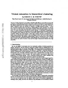
Following is a dendrogram of the results of running these data through the Group Average clustering algorithm. Dendrogram Row 12 11 9 10 8 7 22 19 16 21 20 18 17 15 14 13 6 5 4 2 3 1

8.00

6.00

4.00

Dissimilarity

2.00

0.00

The horizontal axis of the dendrogram represents the distance or dissimilarity between clusters. The vertical axis represents the objects and clusters. The dendrogram is fairly simple to interpret. Remember that our main interest is in similarity and clustering. Each joining (fusion) of two clusters is represented on the graph by the splitting of a horizontal line into two horizontal lines. The horizontal position of the split, shown by the short vertical bar, gives the distance (dissimilarity) between the two clusters. Looking at this dendrogram, you can see the three clusters as three branches that occur at about the same horizontal distance. The two outliers, 6 and 13, are fused in rather arbitrarily at much higher distances. This is the interpretation. In this example we can compare our interpretation with an actual plot of the data. Unfortunately, this usually will not be possible because our data will consist of more than two variables.

Dissimilarities The first task is to form the distances (dissimilarities) between individual objects. This is described in the Medoid Clustering chapter and will not be repeated here.

Hierarchical Algorithms The algorithm used by all eight of the clustering methods is outlined as follows. Let the distance between clusters i and j be represented as d ij and let cluster i contain ni objects. Let D represent the set of all remaining d ij . Suppose there are N objects to cluster. 1. Find the smallest element d ij remaining in D. 2. Merge clusters i and j into a single new cluster, k. 3. Calculate a new set of distances d km using the following distance formula. d km = α i d im + α j d jm + β d ij + γ d im − d jm



NCSS.com


Here m represents any cluster other than k. These new distances replace d im and d jm in D. Also let n k = ni + n j .

Note that the eight algorithms available represent eight choices for α i , α j , β , and γ . 4. Repeat steps 1 - 3 until D contains a single group made up off all objects. This will require N-1 iterations. We will now give brief comments about each of the eight techniques.

Single Linkage Also known as nearest neighbor clustering, this is one of the oldest and most famous of the hierarchical techniques. The distance between two groups is defined as the distance between their two closest members. It often yields clusters in which individuals are added sequentially to a single group. The coefficients of the distance equation are α i = α j = 0.5, β = 0, γ = −0.5.

Complete Linkage Also known as furthest neighbor or maximum method, this method defines the distance between two groups as the distance between their two farthest-apart members. This method usually yields clusters that are well separated and compact. The coefficients of the distance equation are α i = α j = 0.5, β = 0, γ = 0.5.

Simple Average Also called the weighted pair-group method, this algorithm defines the distance between groups as the average distance between each of the members, weighted so that the two groups have an equal influence on the final result. The coefficients of the distance equation are α i = α j = 0.5, β = 0, γ = 0.

Centroid Also referred to as the unweighted pair-group centroid method, this method defines the distance between two groups as the distance between their centroids (center of gravity or vector average). The method should only be used with Euclidean distances. The coefficients of the distance equation are α i =

nj ni ,α j = , β = −α iα j , γ = 0. nk nk

Backward links may occur with this method. These are recognizable when the dendrogram no longer exhibits its simple tree-like structure in which each fusion results in a new cluster that is at a higher distance level (moves from right to left). With backward links, fusions can take place that result in clusters at a lower distance level (move from left to right). The dendrogram is difficult to interpret in this case.

Median Also called the weighted pair-group centroid method, this defines the distance between two groups as the weighted distance between their centroids, the weight being proportional to the number of individuals in each group. Backward links (see discussion under Centroid) may occur with this method. The method should only be used with Euclidean distances. The coefficients of the distance equation are α i = α j = 0.5, β = −0.25, γ = 0.



NCSS.com


Group Average Also called the unweighted pair-group method, this is perhaps the most widely used of all the hierarchical cluster techniques. The distance between two groups is defined as the average distance between each of their members. The coefficients of the distance equation are α i =

nj ni ,α j = , β = 0, γ = 0. nk nk

Ward’s Minimum Variance With this method, groups are formed so that the pooled within-group sum of squares is minimized. That is, at each step, the two clusters are fused which result in the least increase in the pooled within-group sum of squares. The coefficients of the distance equation are α i =

n j + nm − nm ni + n m , γ = 0. ,α j = ,β = nk + nm nk + nm nk + nm

Flexible Strategy Lance and Williams (1967) suggested that a continuum could be made between single and complete linkage. The program lets you try various settings of these parameters which do not conform to the constraints suggested by Lance and Williams. The coefficients of the distance equation should conform to the following constraints α i = 1 − β − α j , α j = 1 − β − α i , − 1 ≤ β ≤ 1, γ = 0. One interesting exercise is to vary these values, trying to find the set that maximizes the cophenetic correlation coefficient.

Goodness-of-Fit Given the large number of techniques, it is often difficult to decide which is best. One criterion that has become popular is to use the result that has largest cophenetic correlation coefficient. This is the correlation between the original distances and those that result from the cluster configuration. Values above 0.75 are felt to be good. The Group Average method appears to produce high values of this statistic. This may be one reason that it is so popular. A second measure of goodness of fit called delta is described in Mather (1976). These statistics measure degree of distortion rather than degree of resemblance (as with the cophenetic correlation). The two delta coefficients are given by  N  * 1/ A  | d jk - d jk |   j