Hierarchical Discriminative Framework for Detecting Tubular ...

Hierarchical Discriminative Framework for Detecting Tubular Structures in 3D Images Dirk Breitenreicher1 , Michal Sofka1 , Stefan Britzen2 , and Shaohua K. Zhou1 1

Imaging and Computer Vision, Siemens Corporation, Corporate Technology, Princeton, NJ, USA 2 Imaging & Therapy Systems, Siemens Healthcare, Forchheim, Germany

Abstract. Detecting tubular structures such as airways or vessels in medical images is important for diagnosis and surgical planning. Many state-of-the-art approaches address this problem by starting from the root and progressing towards thinnest tubular structures usually guided by image filtering techniques. These approaches need to be tailored for each application and can fail in noisy or lowcontrast regions. In this work, we address these challenges by a two-layer model which consists of a low-level likelihood measure and a high-level measure verifying tubular branches. The algorithm starts by computing a robust measure of tubular presence using a discriminative classifier at multiple image scales. The measure is then used in an efficient multi-scale shortest path algorithm to generate candidate centerline branches and corresponding radii measurements. Finally, the branches are verified by a learning-based indicator function that discards false candidate branches. The experiments on detecting airways in rotational X-ray volumes show that the technique is robust to noise and correctly finds airways even in the presence of imaging artifacts.

1

Introduction

Accurate and efficient detection of tree-like structures such as airways or vessels in 3D medical images is important for accurate diagnosis, treatment monitoring, and surgical planning [1,5,8]. The segmentation of such structures is challenging due to noise, imaging artifacts, pathologies, and low-resolution of images (see Fig. 1 for examples). Despite these challenges, the segmented trees are required to be complete and have low number of false branches to make the results accurate for diagnostic and interventional procedures [5,9,15]. In this paper, we propose an efficient algorithm that addresses the challenges above and produces accurate tree detection. This is achieved by discriminative techniques to design a reliable measure of tubularness and to verify candidate branches of the detected tree. State-of-the-art techniques can be roughly categorized into top-down and bottomup. Top-down approaches start at a root point and propagate the tree segmentation into distant branches, for example by region growing [2,9]. These algorithms obtain the segmentation by energy-based image filtering techniques [3,7,13] which evaluate manually tuned cost functions at certain image locations. Strong assumptions on the filter design (e.g. sampling pattern) make it difficult to adapt these algorithms for detecting tubular structures that have high variability of thickness or direction. Furthermore, sophisticated

2 .

. .

.

.

Fig. 1. Accurate detection of airways in rotational X-ray volumes is challenging due to the varying size and context of airways, low signal-to-noise ratio, and presence of imaging artifacts.

stopping criteria are necessary to prevent leaking of the segmentation in regions of high noise, especially when segmenting thin structures and structures of low-contrast. Bottom-up approaches show much more promise [18] and this strategy is also taken in this paper. These algorithms use the likelihood of each voxel belonging to a tubular structure and introduce a tubular neighborhood through a global graph of voxel locations. The tree structure is found through the global optimization on the neighborhood graph that uses candidate source nodes and pre-determined sink node to search for candidate branches. Bifurcations, noisy and low-contrast regions are handled through optimization and graph constraints. Termination criteria are naturally defined by the global optimum of the graph. The challenge is the global optimization which becomes computationally prohibitive with large image sizes. In this work, we present a novel bottom-up algorithm for detecting centerlines and approximate radii of tubular structures. The algorithm relies on a two-layer model which consists of a low-level likelihood measure and a high-level measure verifying tubular branches. The algorithm starts by computing a robust measure of tubular presence using a discriminative classifier at multiple image scales. The classifier responses are then used to identify a number of candidate source points likely belonging to a centerline. The root of the tubular tree (sink) is found in the coarsest scale as a candidate with the highest probability. In the next step, candidate centerline paths from the source points towards the sink are obtained using multi-scale variant of the Dijkstra’s shortest path algorithm. Finally, the candidate paths are verified using a learned branch classifier and combined in a centerline tree. The proposed two-layer model makes it possible to efficiently search for tubular structures in large 3D images. This is because the algorithm only uses the most reliable candidate points (determined at the first layer) to search for centerline paths towards the root. Although a large number of points (several thousand) is used initially, many of them do not yield valid centerlines. These are discarded by the classifier at the second layer which validates the candidate centerline paths. We will show on a dataset of rotational X-ray volumes, that the algorithm effectively detects centerlines of airway trees. Out of all detected centerline points, 74.0% are detected within 4 mm of the ground truth tree centerlines and only 14.3% are detected more than 10 mm away. The final detection speed is 1.5 minutes per volume. The re-

3

sults satisfy clinical requirements and suggest that the approach is suitable for practical use. To the best of our knowledge, this is the first algorithm ever proposed for detecting airway centerlines in rotational X-ray volumes. Extension of the algorithm to other tree-like structures in other modalities should be possible by retraining the classifiers. The paper is organized as follows. After a brief overview of the relevant literature in Sect. 2, the discriminative tubular model is presented in Sect. 3. The two layers of the model are explained in Sect. 3.1 and Sect. 3.2. The experiments on rotational X-ray volumes of the lung are shown in Sec. 4. We conclude the paper in Sect. 5.

2

Related Work

Many centerline extraction algorithms focus on the design of the measure of tubularness at each location. These techniques use intensity values directly, or compute their first or second order derivatives at various locations of a sampling pattern [3,4,7,13]. Such approaches are typically not robust to noise, imaging artifacts, or high variability of tubular sizes and orientations. Furthermore, applying standard multi-scale analysis might not always be possible due to memory and runtime requirements. Finally, some algorithms aggregate measures via a voting mechanism to increase robustness [12,21] but it is not clear how to extract tubular centerlines from the voting maps. The robustness of centerline detectors have been recently improved by applying machine learning techniques. These algorithms model the tubular pattern directly and use discriminative classifiers on features describing low-level image characteristics [5,10,20]. The classifier responses are then used in a region growing algorithm to find the tree segmentations. However, classification solely based on low-level features can have errors due to the absence of contextual information [19]. One approach to model context is to define a graphical model [6,17] which captures the relationships between neighboring locations. These algorithms can be computationally expensive, especially for large volumetric datasets. Standard algorithms used for optimization such as graph cuts or belief propagation can no longer be applied. Another approach is to sample the classification map directly [19] or according to a rotational invariant sampling pattern [17]. The former approach is similar to steerable features which sample the appearance using a regular grid [20]. In our model, we also incorporate context similar to [19,20] but instead of using densely sampled grid, our sampling pattern is specific to centerline branches and thus directly incorporates prior knowledge. Our model has two layers: The first layer models the uncertainty of classifying individual voxels and the second layer decides about tubular branches. A similar idea was used in [6] to segment natural images. The first layer of the hierarchy encodes pixel-wise labeling and the second layer captures relative configuration of objects or parts. However, the distributions are modeled as conditional random fields which are not suitable for tubular objects due to the induced graph topology.

3

Discriminative Tree Detection

Our tree detection algorithm comprises (1) a robust low-level measure of tubularness computed at multiple scales, (2) an efficient bottom-up search strategy, and (3) a reliable

4

Detector 1

… Detector N

Observed Image Y

Prob. density

Branch measure

Final Tree with estimated radius

M scales

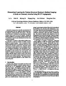
Fig. 2. Automatic detection of tubular structures. In Layer 1 (Sect. 3.1), the density p(xi |Y ) is obtained using N detectors at each of the M scales. In Layer 2 (Sect. 3.2), the candidate centerlines are verified using the branch measure p(Bi |b(Xi )) to compose the final centerline tree.

branch verification. The low-level measure indicates the presence of a tubular structure at each voxel location. The measure is determined by a discriminative classifier trained on a large annotated database of images (Sect. 3.1). The likelihood measure is used in a multi-scale centerline extraction procedure based on Dijkstra’s shortest path search. This step produces promising candidate branches of a tree (Sect. 3.2). The candidate branches are verified using a discriminative classifier which prunes false branch candidates while preserving true branches. Finally, an approximate tube radius is estimated at each centerline point. The algorithm stages are shown in Fig. 2. Let each tubular tree be composed of constituent tubular structures. The centerlines of tubular structures are detected using a hierarchical model as follows. Let C = {B1 , . . . , Bn } denote a centerline composed of branches Bi , i = 1, . . . , n. Each branch Bi consists of centerline points Xi = x1 , x2 , ..., xn . In our case, xi = {xl , xs } denotes a point location xl and size (radius) xs . The observations Y are obtained by extracting features for each centerline point xi from an image neighborhood at scale xs surrounding location xl . The goal of the centerline extraction is to obtain C ∗ maximizing the posterior probability p(C|Y ) over all centerlines C. Clearly, this optimization is computationally involved in most practical situations due to the large space of centerlines. Therefore, we consider a posterior approximation which is based on the assumption that the branches are pairwise independent: p(B1 , . . . , Bn |Y ) =

n Y

p(Bi |Y ) .

(1)

i=1

Although this assumption ignores the connectivity of branches Bi , we will show that (1) empirically yields accurate centerline detections. Next, since each branch Bi consists of centerline points Xi ∈ X , we can write (1) as X p(Bi |Y ) = p(Bi |Xi )p(Xi |Y ) , (2) Xi ∈X

where p(Xi |Y ) refers to the posterior distribution of centerline points given image observations. Inferring the optimal set of branches from (2) is possible using e.g. Monte

5

Carlo sampling strategies [14]. However, in our setting, the large domain of X prohibits the application of exhaustive sampling. In order to efficiently find the optimal set of branches, we propose a two layer model, inspired by the hierarchical field applied to segmentation of natural images [6]. The optimal configuration and the uncertainty obtained from p(Xi |Y ) at the first layer is propagated to the second layer. The second layer infers the centerline from branch candidates and their corresponding uncertainties. The overall algorithm is shown in Fig. 2. Formally, let the probability density at each site xi be represented as bi (xi ) = p(xi |Y )

(3)

and the set of branch probabilities be expressed as b(Xi ) = {bi (xi )}xi ∈Xi .

(4)

Xi∗

Then, the optimal configuration of tubular centerline points can be obtained by site-wise maximization of b(Xi ). As a consequence, we can approximate (2) [6] by
p(Bi |Y ) ≈ p Bi |b(Xi ) . (5) Both layers, i.e. the computation of the branch location probabilities in (4) and the inference of branches in (5), will be described in detail next. 3.1

Layer 1: Multi-Scale Voxel-Wise Detection

In this section, we describe how to estimate the conditional density p(xi |Y ). This term determines the likelihood of a voxel location being a tubular structure given observations. We train a Probabilistic Boosting Tree classifier (PBT) [16], that has nodes composed of AdaBoost classifiers trained to select features that best discriminate between positive and negative examples of the tubular structures. Let us now define a random variable y ∈ {−1, +1}, where y = +1 indicates presence and y = −1 absence of the tubular structure. The PBT classifier is trained to select features that best discriminate between positive and negative samples. We can then evaluate the probability of a tubular structure being detected as p(yi = +1|xi , Y ) and therefore rewrite the density as p(xi |Y ) = p(yi = +1|xi , Y ) .

(6)

The classifiers are extracted for M different scale levels which correspond to the sizes of tubular structures. This multi-scale setup has several advantages compared to a classifier trained at a single scale. First, it provides more accurate results by training more focused classifier since the structures at each scale have different anatomical context (see Fig. 1). Second, robustness is improved since the feature parameters are adjusted for each scale level rather than using one set of parameters for all tubular structure sizes. Third, no special treatment is necessary to ensure uniform distribution of samples of different tubular sizes which would otherwise be needed since a typical tree contains more thin than thick branches. The classifiers at each scale level use 3D Haar features. The advantage of Haar features (apart from being efficient to compute) is that they form a basis and can approximate first and second order differential operators with only few basis elements. As such they can naturally mimic more complicated features such as Hessian or Flux [7,13].

6

M scales

Fig. 3. In the standard Dijkstra’s algorithm (left), the shortest path (blue) is obtained using a single level (which could be composed from multiple scales) by tracing the high probability regions (black and dark grey). In the multi-scale variant (right), the tracing is performed over multiple scales M . The cost penalties on scale changes make it possible to avoid exploring unnecessary regions which results in faster computation and higher robustness.

3.2

Layer 2: Branch Measure


The conditional density of the branch p Bi |b(Xi ) is estimated using a set of candidate branches and the associated branch probabilities (4). The candidate branches are extracted by the shortest path tracing algorithm as follows. Let a candidate centerline branch originate from a source vertex s of G and terminate at the root vertex v (both automatically determined as described below). We associate each voxel with a vertex and we assume that each voxel is connected by an edge to its 18 neighbors. Let c be a nonnegative cost assigned to each edge and computed from
2 the voxel-wise classifiers specific for each scale M using (4) as: c = 1 − bi (xi ) . The single-source shortest path is then computed by finding, for a vertex v reachable from s, the minimum-cost path from s to v. We perform the search by a multi-scale variant of Dijkstra’s shortest path algorithm as illustrated in Fig. 3. Since the tubular size along the path generally increases, we set the costs to 0 and ∞ for switching from a fine to a coarse level and from coarse to fine, respectively. This way, the centerline branches Bi are extracted by following high values of bi over M scales. The source vertex points are generated as follows. The probability density maps obtained from (6) are combined by computing the maximum over scales. The combined map is used as input to a skeletonization algorithm [11]. The skeleton points serve as source point samples which might contain many false centerline points but cover all branches. The sink vertex point is computed as the point with the highest probability after applying skeletonization at the coarsest level. This is robust due to the distinctiveness of the trachea. The shortest path is found between each source point s and a vertex point v (which can be the root point or any previously detected centerline point). This way, bifurcations are handled simply by connecting branches.
Each branch is assigned a probability using the density p Bi |b(Xi ) from (5). Only high probability branches are kept and merged into the final centerline tree. The density
p Bi |b(Xi ) is obtained from a discriminative classifier similar to (6). As features, we extract various statistics from Bi , i.e. the average, minimum and maximum intensity and

7

likelihood, histogram distributions of the local intensity and likelihood, distribution of the tubularness measures from [4], and the distribution of scale values, which all focus on the local context of Bi . The most discriminative features were average intensity (used 17% of the time), average likelihood (14%), and minimum likelihood (8%). From the distributions, tubular features were used most often. To introduce characteristics which take the entire branch into account, we extract a piece-wise linear approximation L of Bi up to a given accuracy and use the number of piecewise elements in L, the minimum, maximum, and average angular change between elements in L, and the absolute length of L.

4

Experiments

Before discussing the experiments, the training procedure is first described in Sect. 4.1. The experimental evaluation in Sect. 4.2 starts by a comparison of various features used as a measure of tubularness (Layer 1), which includes learning-based techniques. The next experiments compare qualitatively and quantitatively the detected centerlines to ground truth. Finally, a set of testing images is used to compute statistics of overall centerline detection errors and radius deviations. 4.1

Training the Tubular Model

Experts annotated a database of medical images by connecting airway centers and assigning approximate airway radii while navigating the visualization planes of each image. The annotated database is leveraged to train both layers of the tubular model. The Layer 1 is trained at M = 3 scale levels. At the three levels, the diameter of tubular structures are 1.5 to 3.5 mm, 3.0 to 7.0 mm, and 6.0 to 30.0 mm to handle thin, medium and large airways respectively. At each scale level, we train a sequence of N = 3 Probabilistic Boosting Tree (PBT) classifiers [16] using a tree depth of 3 and 10 weak learners at each level. To train the branch measure at Layer 2, we generate the set of positive samples (true branches) and negative samples (false positives) as follows. First, we run Layer 1 detection on a separate training dataset and obtain source points as described in Sect. 3.2. The source points are used to run tracing by applying Dijkstra’s shortest path. This way, we obtain set of branch samples. The samples are labeled as positives, if they have no more than 7 centerline points outside (with 1 voxel tolerance) of the ground truth tubular structure. Otherwise, they
are labeled as negatives. The samples are used to train the branch measure p Bi |b(Xi ) using PBT classifiers with tree depth of 4 and 20 weak learners at each level. 4.2

Airway Trees in Rotational X-ray

Our data set consists of 49 rotational X-ray volumes of the lung acquired by an Axiom Artis imaging system from Siemens. The system is useful during interventions since it provides full 3D acquisition at lower radiation and faster scanning time compared to standard CT but the images are noisy and contain various imaging artifacts. The

8 1 Haar Steerable Flux Hessian Flux−filter Frangi−filter

True Positive Rate

0.95

0.9

0.85

0.8

0.75

0

0.05

0.1

0.15

0.2

0.25

False Positive Rate

Fig. 4. ROC plots computed for the voxel classification using p(xi |Y ) from Layer 1. The plots are computed for the learning-based classification (using Haar, steerable [20], flux [7], and intensity Hessian features) and for the filter-based techniques using flux filter [7] and Frangi filter [4]. Learning-based classification using Haar features performs the best. Example of a response combined over scales is shown for one coronal slice on the right.

volumes have resolution 0.40 × 0.49 × 0.49 mm3 and average size of 512 × 512 × 275. A total of 36 volumes are used for training and 13 for testing (selected randomly). The first experiment evaluates the performance of Layer 1 (Fig. 4). The model was trained as described in Sect. 4.1 and applied to unseen cases. The resulting probability density (6) was thresholded at various levels between 0 and 1. This produced voxel-wise classification of airways. We compared learning-based classification (using Haar, steerable [20], flux [7], and intensity Hessian features) and filter-based techniques (using flux filter [7] and Frangi filter [4]). Learning-based classification using Haar features performs the best. Although Haar features are simpler than tube-specific filters, combination of different Haar types in the classification can learn complex patterns. The next experiments compares the detected centerlines to the ground truth annotation. This is done by computing for each centerline point the Hausdorff distance to the ground truth centerline tree. The distance is shown on the detected tree by color coding the centerlines. This shows, for each point and branch on the detected tree, how far it is w.r.t. the ground truth tree (evaluating true positives and false positives). The same procedure is repeated for each ground truth centerline point by computing Hausdorff distances to the detected tree. This evaluates false negatives. Fig. 6 shows example results for the cases in Fig. 5. Overall, there is a good agreement of the detected tree and the ground truth tree. Both trees show only several points marked as red demonstrating low false positive and false negative detection, respectively. This is possible by the proposed branch measure which uses many candidate centerlines (and their uncertainties) to reject false positives (Fig. 7). The final experiment shows quantitative evaluation of all detected centerlines. As before, we compute the Hausdorff distance for each centerline point on the detected and on the ground truth tree, respectively. The distances are then plotted in two histograms, one for the detected and one for the ground truth tree (Fig. 8). The plots show that 40.8% of detections are within 1 mm, 60.5% within 2 mm, and 74.0% of all centerline

9

Case 1

Case 2

Case 3

Fig. 5. Detection result (red) on unseen cases. Ground truth annotation is marked as green. Note that since the intersection of the airways and the visualization plane can have various angles, the boundaries are not always circular. The image on the right only contains one lobe. All images show high level of noise.

points are within 4 mm of the ground truth. There are only 14.3% centerline points detected more than 10 mm from the ground truth. Correspondingly, there are 44.0%, 65.0%, and 77.8% ground truth centerline points within 1, 2, and 4 mm of detected centerlines, respectively. Only 13.0% ground truth centerline points are more than 10 mm from the detected tree. The detected centerlines have radius error within 1 mm of ground truth for 79.1% points. Please note, that this strict evaluation is performed at the centerline level rather than the branch level as in [5], for example. Despite that, the results suggest that the algorithm is suitable for clinical setting, e.g. for bronchoscopic navigation [5,15], since most detected centerlines are within the airway boundaries. The tree extraction algorithm is efficient. Computing the multi-scale likelihood maps takes on average 1.5 minutes per volume on Intel Xeon 2.67 GHz computer. Significant improvement is possible by computing the maps only in local regions determined from the neighborhood surrounding the source and sink points. The candidate branches are extracted in less than 1 second on average. Finally, the branches are verified in less than 1 second on average yielding fast overall computational speed.

5

Conclusion

In this work, we presented a discriminative approach for automatic detection of tubular structures from volumetric datasets. The algorithm is robust and efficient thanks to the two-layer model of tubular centerlines and associated tubular sizes. Layer 1 provides an indication of how likely a particular voxel location belongs to a tubular structure. The most likely locations and the automatically determined tree root are used to find candidate centerline branches using a multi-scale variant of Dijkstra’s shortest path algorithm. The candidate branches are verified at Layer 2 by a discriminative branch measure. The algorithm was evaluated on a challenging dataset of rotational X-ray volumes of the lung – the first reported technique for this type of dataset. The airway centerlines were accurately detected with as much as 77.8% centerline points being within 4 mm

Case 3

Case 2

Case 1

10

Fig. 6. Tree detection result (left) compared to ground truth annotation (right) on images from Fig. 5. Color reflects the point-wise Hausdorff distance of each centerline point to the reference tree. For the left column, the reference tree is ground truth and for the right column, the reference tree is the detection. Note the agreement of the detection and ground truth as evidenced by low number of red branches on the left (low false positives) and on the right (low false negatives). Case 3 had only image acquisition of one lobe.

11

Fig. 7. Example of branch pruning using the proposed branch measure. For the automatically detected tree (left) false branch candidates (red) are rejected to obtain a verified estimate (right).

Fig. 8. Overall detection errors summarized as a histogram of Hausdorff distances for all testing cases. The left plot shows the relative distribution of distances from the detected result to ground truth (blue) and vice versa (red). The right plot shows the corresponding errors of tubular radius estimation.

of correponding ground truth annotation and with radius error of less than 1 mm for 79.1% of the points. Our future work will focus on improving accuracy, especially for thin structures. This will require feature computation at a subvoxel level which will pose a challenge in keeping the computational speed fast. In addition, we will explore the use of treeprior information to further boost the robustness and accuracy. We also plan to design an additional data-driven boundary refinement step to improve the accuracy of tubular radius estimation. Finally, we would like to verify the algorithm on other applications, e.g. detecting vessels in liver scans.

12

References 1. Barbu, A., Bogoni, L., Comaniciu, D.: Hierarchical part-based detection of 3d flexible tubes: Application to ct colonoscopy. In: Proc. Int. Conf. Med. Imaging Comp. and Comp. Assisted Intervention. pp. 462–470. Springer (2006) 1 2. Bauer, C., Pock, T., Sorantin, E., Bischof, H., Beichel, R.: Segmentation of interwoven 3D tubular tree structures utilizing shape priors and graph cuts. Med. Image Anal. 14(2), 172– 184 (2010) 1 3. Benmansour, F., Cohen, L.D.: Tubular structure segmentation based on minimal path method and anisotropic enhancement. Int. J. Comput. Vision 92, 192–210 (2011) 1, 3 4. Frangi, A., Niessen, W., Vincken, K., Viergever, M.: Multiscale vessel enhancement filtering. In: Proc. Int. Conf. Med. Imaging Comp. and Comp. Assisted Intervention (1998) 3, 7, 8 5. Graham, M., Gibbs, J., Cornish, D., Higgins, W.: Robust 3-d airway tree segmentation for image-guided peripheral bronchoscopy. IEEE T. Med. Imaging 29, 982–997 (2010) 1, 3, 9 6. Kumar, S., Hebert, M.: A hierarchical field framework for unified context-based classification. In: Proc. Int. Conf. Comput. Vision (2005) 3, 5 7. Lesage, D., Angelini, E., Bloch, I., Funka-Lea, G.: Design and study of flux-based features for 3D vascular tracking. In: Proc. Int. Symp. Biomed. Imaging (2009) 1, 3, 5, 8 8. Lesage, D., Angelini, E., Bloch, I., Funka-Lea, G.: A review of 3D vessel lumen segmentation techniques: Models, features and extraction schemes. Med. Image Anal. 13(6), 819–845 (2009) 1 9. Lo, P., Sporring, J., Ashraf, H., Pedersen, J.J., de Bruijne, M.: Vessel-guided airway tree segmentation: A voxel classification approach. Med. Image Anal. 14(4), 527 – 538 (2010) 1 10. Ochs, R., Goldin, J., Abtin, F., Kim, H., Brown, K., Batra, P., Roback, D., McNitt-Gray, M., Brown, M.: Automated classification of lung bronchovascular anatomy in CT using AdaBoost. Med. Image Anal. 11, 315–324 (2007) 3 11. Pal´agyi, K., Sorantin, E., Balogh, E., Kuba, A., Halmai, C., Erdohelyi, B., Hausegger, K.: A sequential 3D thinning algorithm and its medical applications. In: Proc. Int. Conf. on Information Processing in Med. Imaging. pp. 409–415. London, UK (2001) 6 12. Rouchdy, Y., Cohen, L.: A geodesic voting method for the segmentation of tubular tree and centerlines. In: Proc. Int. Symp. on Biomed. Imaging. pp. 979–983 (2011) 3 13. Schuh, A., Kaftan, J.N., Tietjen, C., O’Donnell, T.P.: Sparse axes-aligned MFlux. In: Workshop on Comp. and Vis. for (Intra-) Vascular Imaging (2011) 1, 3, 5 14. Sofka, M., Zhang, J., Zhou, S., Comaniciu, D.: Multiple object detection by sequential Monte Carlo and hierarchical detection network. In: Proc. Int. Conf. Comput. Vision and Pattern Recogn. San Francisco, CA (13–18 Jun 2010) 5 15. Steger, T., Hosbach, M.: Navigated bronchoscopy using intraoperative fluoroscopy and preoperative CT. In: Proc. Int. Symp. on Biomed. Imaging. pp. 1220 –1223 (2012) 1, 9 16. Tu, Z.: Probabilistic boosting-tree: learning discriminative models for classification, recognition, and clustering. In: Proc. Int. Conf. Comput. Vision (2005) 5, 7 17. Tu, Z., Bai, X.: Auto-context and its application to high-level vision tasks and 3D brain image segmentation. IEEE Trans. Pattern Anal. Machine Intelligence 32, 1744–1757 (2010) 3 18. T¨uretken, E., Benmansour, F., Fua, P.: Automated reconstruction of tree structures using path classifiers and mixed integer programming. In: Proc. Int. Conf. Comput. Vision and Pattern Recogn. pp. 566–573. IEEE (2012) 2 19. Wolf, L., Bileschi, S.: A critical view of context. Int. J. Comput. Vision (2006) 3 20. Zheng, Y., Loziczonek, M., Georgescu, B., Zhou, S.K., Vega-Higuera, F., Comaniciu, D.: Machine learning based vesselness measurement for coronary artery segmentation in cardiac CT volumes. In: Proc. SPIE (2011) 3, 8 21. Zhou, J., Chang, S., Metaxas, D., Axel, L.: Vascular structure segmentation and bifurcation detection. In: Proc. Int. Symp. on Biomed. Imaging. pp. 872–875 (2007) 3