define and provide an effective solution for the hierarchical power management
..... request AIATs of the ith type of application as the input feature. , in which.
Hierarchical Dynamic Power Management Using Model-Free Reinforcement Learning Yanzhi Wang1, Maryam Triki2, Xue Lin1, Ahmed C. Ammari23, Massoud Pedram1 1 Department of Electrical Engineering, University of Southern California, Los Angeles, CA USA 2 National Institute of the Applied Sciences and Technology (INSAT), Carthage University, Tunisia 3 Department of Elec. & Computer Engineering, King Abdulaziz University, Jeddah, Saudi Arabia E-mail:
[email protected] Abstract Model-free reinforcement learning (RL) has become a promising technique for designing a robust dynamic power management (DPM) framework that can cope with variations and uncertainties that emanate from hardware and application characteristics. Moreover, the potentially significant benefit of performing application-level scheduling as part of the system-level power management should be harnessed. This paper presents an architecture for hierarchical DPM in an embedded system composed of a processor chip and connected I/O devices (which are called system components.) The goal is to facilitate saving in the system component power consumption, which tends to dominate the total power consumption. The proposed (online) adaptive DPM technique consists of two layers: an RL-based component-level local power manager (LPM) and a system-level global power manager (GPM). The LPM performs component power and latency optimization. It employs temporal difference learning on semi-Markov decision process (SMDP) for model-free RL, and it is specifically optimized for an environment in which multiple (heterogeneous) types of applications can run in the embedded system. The GPM interacts with the CPU scheduler to perform effective application-level scheduling, thereby, enabling the LPM to do even more component power optimizations. In this hierarchical DPM framework, power and latency tradeoffs of each type of application can be precisely controlled based on a user-defined parameter. Experiments show that the amount of average power saving is up to 31.1% compared to existing approaches.
Keywords Dynamic power management, reinforcement learning, Bayesian classification
1. Introduction Dynamic power management (DPM), which refers to the selective shut-off or slow-down of system components that are idle or underutilized, has proven to be a particularly effective way of reducing power dissipation at system level [1]. Bona fide DPM frameworks should consider variations that originate from process, voltage, and temperature (PVT) variations as well as device aging, current stress, and interconnect wear-out in the underlying hardware. They should also account for workload type and intensity variations. In addition, robust DPM frameworks must also *This research is sponsored in part by a grant from the National Science Foundation.
cope with sources of uncertainty in the system under their control, e.g., inaccuracies in monitoring data about the current state of the system. The sources of variability and uncertainty tend to cause both the difficulty of determining the current state of the system and predicting the next state given DPM agent’s action, and the difficulty in determining the reward rate of a chosen or contemplated action. The DPM methods proposed in the literature [1]-[13] can be broadly classified into three categories: ad hoc, stochastic, and learning based methods. Ad hoc policies [2][3] are based on the idea of predicting whether the next idle period length is greater than the break-even time . They perform well only when the requests are highly correlated, and do not take system performance into account. By modeling the request arrival times and device service times as stationary stochastic processes, stochastic DPM policies can take into account both power and performance. They can also compute the exact solution for the performance-constrained power optimization problem. In [4], Benini et al. model a power-managed system as a discrete-time Markov decision process (MDP) by assuming that the service time of a request follows a geometric distribution. Qiu et al. in [5] model a similar system by using a continuous-time MDP. This in turn enables the power manager (PM) to work in an event-driven manner, thereby reducing the decision making overhead. Other enhancements include time-indexed semi-MDP [6]. In all the stochastic DPM approaches, request inter-arrival times and system service times are modeled as stationary processes that satisfy certain probability distributions. In addition, an optimal policy for the given MDP can be found only if we have knowledge of the state transition probability function and reward function of the MDP. Reinforcement learning is primarily concerned with how to obtain the optimal policy for a MDP when such a model is not known a priori. The DPM agent must interact with environment to obtain information which, by means of an appropriate algorithm, can be processed to produce an optimal policy. Several recent work use machine learning for adaptive policy optimization. Compared to ad hoc policies, machine learning-based methods can simultaneously consider power and performance, and perform well under various workload conditions. In [7], an online policy selection algorithm is proposed, which generates offline a set of DPM policies to choose from. The effectiveness of the learning algorithm depends heavily on DPM policy selection. Tan et al. in [8] propose to use an enhanced Q-learning algorithm for system-level DPM. This is a model-free RL
approach since the PM does not require prior knowledge of the state transition probability function, while the knowledge of the state and action spaces and also the reward function is required. The Q-learning based DPM learns a policy online by trying to learn which action is the best for a certain system state, based on the reward or penalty received. In this way the PM does not depend on any pre-designed experts, and it can achieve a much wider range of power-latency tradeoffs. However, this work is based on discrete-time model of the stochastic process, and thus has large decision making overhead. Therefore Wang et al. in [9] extend this work to enable the PM to work in a continuous-time and event-driven manner with fast convergence rate, by exploiting the TD(λ) learning framework for semi-MDP (SMDP) [14]. Moreover, workload prediction based on a Bayesian classifier [16] is also incorporated in this work to provide partial information about the state of the service request (SR) generation so that the RL algorithm can work effectively in a partially observable environment. All of the above-mentioned DPM works have focused on developing local component-level policies without differentiating between the service request characteristics of various software applications, and therefore, they have ignored the potential benefit of performing application-level scheduling as part of the system-level power management [10]. Application-level scheduling requires the PM to have a global view of the system architecture and work closely with the operating system scheduler. These are beyond the capabilities of the aforesaid DPM solutions. Therefore we define and provide an effective solution for the hierarchical power management problem by providing (i) an RL-based local power manager (LPM) for the system component, which is more effective and robust to variations and uncertainties than that proposed in [9], and (ii) a systemlevel global power manager (GPM), which performs application-level scheduling, thereby enhancing the component-level power optimizations. A few research results related to the hierarchical power management have been reported. Reference [11] uses a similar system set-up as this paper, and provides optimal solution for a computer system with self power-managed components by assuming a continuous-time MDP model given in advance for the power management system. However, this assumption may not be realistic. Reference [12] proposes a hierarchical adaptive DPM, where the term “hierarchical” refers to the manner in which the authors formulate the DPM policy optimization as a problem of seeking an optimal rule that switches policies among a set of pre-computed ones. The contribution of this paper is twofold. First, we enhance the RL-based DPM policy proposed in [9] for the local component by improving the state and action spaces of the RL algorithm, as well as making other improvements for handling multiple types of user applications. Moreover, the LPM still offers the following benefits: it is model-free, independent of pre-designed policies, performs learning and power management in a continuous-time and event-driven manner, has fast convergence rate and less reliance on the Markovian property, and is capable of performing precise
power-latency tradeoff based on a user-defined parameter. Workload prediction based on online Bayesian classifier is also incorporated to provide partial information about the service request state for the LPM. The second part of our contribution is the development of a GPM that performs effective application-level scheduling, thereby, helping the LPM achieve more component-level power optimizations. The fairness issue related to distributing execution times among various software applications is also taken care of by the GPM. Experiments on measured data traces demonstrate the superior performance of the proposed hierarchical power management method compared with prior works [7][9].
2. Theoretical Background 2.1. Temporal Difference Learning for SMDP In this section we provide a brief introduction of the general RL framework and the RL algorithm proposed for the LPM, named the TD( ) learning algorithm for SMDP. As illustrated in Figure 1, the general RL model consists of an agent, a finite state space , a set of available actions , and a reward function . A policy is a set of state-action pairs for all states in the RL framework. We use notation to specify the action chosen in state according to policy . We consider the class of deterministic policies in this work.
Figure 1: Agent-environment interaction model. Assume that the agent-environment interaction system is continuous in time but has a countable number of events. Then there exists a countable set of times , known as epochs. At epoch , system has just transitioned to state . The agent selects an action according to some policy . At time , the agent finds itself in a new state , and, in the time period , it receives a scalar reward with rate . We define the return as the discounted integral of reward rate, whenever a selection of action is made by the agent. Obviously, both the policy and the agent-environment interaction model are assumed to be stationary for the proper definition of the return . We define the value of a state-action pair under a policy , denoted by , as the expected return when starting from state , choosing action (according to the policy ), and following thereafter. An optimal policy is the one maximizing the value functions for all state-action pairs. For a realistic RL algorithm, the agent (power manager) has no predefined policy or knowledge about state transition characteristics (which are essential in the stochastic DPM approaches.) Therefore the agent has to simultaneously learn the optimal policy, and use that policy to control (make decisions.) Traditional value iteration or policy iteration methods cannot be applied here. Instead the temporal
difference (TD) learning method [15] for SMDP may be used. Such method generates an estimate for each state-action pair at epoch , which is the estimate of the actual value following policy . Suppose that state is visited at epoch , then at that epoch the agent chooses an action either with the maximum estimated value for various actions , or by using other semi-greedy policies [15]. Moreover, the TD learning rule updates the estimate at the next epoch , based on the chosen action , and the next state . Various TD learning algorithm implementations are mainly different from one another by their updating (evaluating) methods. We choose to use the TD( ) algorithm for SMDP [14] due to a joint consideration of effectiveness, robustness and convergence rate. More specifically, the value update rule for a state-action pair at epoch in the TD( ) algorithm for SMDP is computed as follows: (
)
In the above expression, system remains in state ; rate;
is the discount factor;
∏ as follows:
∏
,
(4)
In the original algorithm, the prior and conditional probabilities are obtained by performing Maximum Likelihood estimation on the whole data set. However, in this work we have to implement the predictor in an online fashion. So when we observe a sequence of features and output , we update the conditional and prior probabilities as follows: (5) where
denote the updating rate parameters.
3. Hierarchical DPM Framework
(1)
is the time that denotes the learning is the sample
discounted reward received in time units; is the estimated value of the state-action pair in which is the actually occurring next state. Moreover, in Eqn. (1) denotes the eligibility of each state-action pair , to facilitate the implementation of the TD( ) algorithm. Such eligibility reflects the degree to which the state-action pair has been chosen in the recent past. It is updated as follows: ( ) (2) where
We have and we compute the MAP class of
denotes the delta kronecker function.
2.2. Online Bayesian Classifier Naïve Bayesian classifier is a generative classifying technique using the idea of maximum a posteriori (MAP). It is selected as the workload predictor in the proposed hierarchical DPM framework because of its relatively high prediction rate, as well as the fact that the partial information it provides contains certain degree of certainty due to the use of posterior probability. Given input feature , the classifier’s goal is to assign class label from set for the output , by maximizing the posterior probability : (3) where the denominator is the same for every class assignment of . ), which is the prior probability that the class of is , can be calculated from the training set. Hence, we only need , the conditional probability of seeing the input feature vector given that the class of is . A fundamental assumption of Bayesian classifier made is that all input features are conditionally independent given class , e.g., .
Figure 2: Block diagram of the hierarchical DPM structure. We consider a specific I/O device (component), e.g., hard disk, WLAN card, or USB devices, in a uni-processor embedded system. Batches of applications keep running on the system. When an application is running on the CPU, it may send requests to the I/O device for services. It is also required that each type of application gets a fair share of CPU time over a long period of time. In this paper we shall focus on reducing power consumption and finding a nearoptimal power-latency tradeoff of the I/O device in the system. The architecture of the proposed hierarchical DPM framework is presented in Figure 2. When the CPU is running applications, it generates requests through a service requestor (SR), and pushes the requests through a service queue (SQ) if they have to wait for processing. The exact generating time instances of service requests are not known a priori. The component or service provider whose power is being managed is denoted by SP in this figure. Active
Idle
Transition to active
Transition to sleep
Sleep
Figure 3: State diagram of SP. The service provider (SP) has three main states as shown in Figure 3. It is in the active state while processing services, and after it has finished, it becomes idle. The SP can autonomously and instantaneously transit to active state as soon as any task arrives. Unfortunately, the SP has non-zero power consumption in idle state. It can, however, go to the
sleep state from the state. A sleeping SP consumes little power compared to an idle one, but it suffers from large wakeup latencies along with high power consumption during the transition to active state. Our goal is to properly schedule the sleep time for the SP in order to reach the balance between latency and energy consumption. As shown in Figure 2, the proposed DPM framework has two levels of PM. In the system level, the GPM acts as the central controller which attempts to meet certain performance (latency) constraint for the component while minimizing the component power consumption. The GPM works with the CPU scheduler to select the right applications to run so as to reduce the component power dissipation, while taking into account the fairness issues among different types of applications. This decision is in turn made based on the current state of the power management system, including the state of the SP, the number of requests waiting in the SQ, etc. Note that in this architecture, the GPM cannot directly control the state transition of the SP, and therefore performing application scheduling is the method that the GPM uses to guide the local PM policy and improve the power efficiency of the SP. In the component level, the SP, i.e., the I/O device, is controlled by the LPM. The LPM is based on the one proposed in [9] using RL-based DPM algorithm, with both enhancements on the state-action spaces of the RL algorithm, as well as other enhancements for the hierarchical power management framework. The LPM monitors the current type of application running in the CPU, the number of requests waiting in the SQ, the (estimated) current state of SR (i.e., the service request generating rate), the current SP state (active, idle, sleep, etc.), and consequently makes decisions (adjusts the state of the SP.) There are two decision points for the LPM: First, every time the SP transits from active to idle state, the LPM will make a decision on whether to let the SP go to sleep straightaway or set a timeout. If a timeout is set and no requests arrive during this period, the device will subsequently go to sleep. Second, while SP is in the sleep state, the LPM decides whether or not to wake up the SP based on the number of waiting requests in the SQ. To be more realistic, we consider in this work that the exact SR state cannot be directly obtained by the LPM, and the LPM also has no prior knowledge of the characteristics of the SR. Therefore, workload prediction has to be incorporated to provide partial information (estimation) of the SR state to the LPM so that the LPM can effectively learn in the observation domain of SR. We adopt the aforesaid online Bayesian predictor (BP) for workload prediction, as shown in Figure 2.
4. Hierarchical DPM Algorithm In this section, we explain how to extend RL techniques to solve the hierarchical power management problem, in three aspects: the workload prediction using online Bayesian predictor, the LPM, and the GPM. We first introduce several definitions and notations. Suppose that the whole system begins operating at time , and we are currently at time instance . Suppose there are types of applications in the hierarchical framework, and we let denote the type of application running
in the CPU at time . Furthermore, we use to denote the actual generation time (AGT), i.e., the actual time instance that such request is generated by the SR, of the jth request of the ith type of application. Then the application-specific generation time (ASGT) of the jth request of the ith type of application, denoted by , is defined by the following: ]
∫
(6)
where ] is the indicator function which equals to one if the Boolean variable is true, and otherwise equals to zero. Finally, the application-specific inter-arrival time (AIAT) of two consecutive service requests, say, the jth and the (j+1)st, of the ith type of application, is given by .
4.1. Online Bayesian Predictor The proposed system relies on workload prediction method to provide partial observation of the actual SR state for the LPM. Previous work on workload prediction in [2][3] assumes that a linear combination of previous idles times (or request inter-arrival times) may be used to infer the future ones, which is not always true. For example, one very long inter-arrival time can ruin a set of subsequent predictions. Thus an online naïve Bayesian classifier, which can overcome the above effect and result in much higher prediction accuracy, is adopted as the workload predictor. We use online Bayesian predictors, each corresponding to a specific type of application. Consider a specific ith Bayesian predictor corresponding to the ith application type. We use characteristics of the previous request AIATs of the ith type of application as the input feature , in which if the corresponding interval length is greater than the break-even time ; otherwise . The output is the prediction whether or not the next AIAT is greater than . In real implementations, we use three output states “long, short, and unknown”. We predict the next AIAT to be “unknown” if the difference between the posterior probabilities that the next AIAT is long and that it is short is less than a predefined parameter .
4.2. The Local Power Manager
Figure 4: Component model and local power manager. The component whose power is being managed by LPM is shown in Figure 4. Suppose that we are currently at time , and the ith type of application is running. We assume that ∫
]
(7)
Then the state parameters at time of the power managed component monitored by the LPM are the following four: The type of application running in CPU, i.e., .
The SP state , which is the component power state (active, idle, sleep, etc.). The SQ state , which is the number of requests in the SQ. The estimated SR state, which is represented in this paper by the estimation (long, short, unknown, etc.) on the AIAT of the ith type of application from th the i online Bayesian predictor. To apply RL techniques in the LPM, we define decision epochs, i.e., when new decisions can be made and updates for RL algorithm can be executed. In our case, the decision epochs coincide with one of the following three cases: 1. The SP entered idle state ( = idle) and = 0. 2. The SP has just entered the sleep state and finds that > 0. 3. The SP is in sleep state and a new request arrives. We further denote the kth decision epoch of the ith type of application by . There are mainly two types of decision epochs. If at decision epoch , we have = idle and = 0 (case 1), we call the decision epoch an idlestate decision epoch, denoted by . On the other hand, if at decision epoch , we have = sleep (case 2 or case 3), we call decision epoch a sleepstate decision epoch, denoted by . In this work we adopt a more general power management framework in which each type of application may have its own performance degradation constraint (which implies that different types of applications may have different constraints), defined as the constraint on the average latency per request of that specific type of application. Therefore the proposed DPM framework should minimize the average component power consumption for each type of application, while satisfying its performance degradation constraint. Note that this requirement cannot be satisfied in the reference machine learning based DPM works [7][8][9]. In this paper, we should be able to control the power-latency tradeoff of each type of application separately, in order to satisfy the requirement. Therefore, it necessitates the following constraint on CPU scheduling: Application type switch, i.e., the changing of application type running in the CPU, can only occur at idle-state decision epochs of the RL algorithm used in the LPM. Due to the previous CPU scheduling constraint, we “split” each decision epoch into two sub-decision epochs and . We assume that at sub-decision epoch , decisions are made by the RL algorithm used in the LPM; while at sub-decision epoch , updates in the RL algorithm are executed. We have , i.e., at each decision epoch, updates are performed first and subsequently new decisions are made. Due to the previous CPU scheduling constraint, no application type switch can happen within the time period . Or equivalently, there are no other sub-decision epochs of any type of application within the time period . Suppose that we are now at sub-decision epoch , and the LPM makes a decision and issues a command to execute it. Due to the previous assumption of the CPU scheduler,
there will be no application type switch until the next subdecision epoch , which belongs to the same type of th application (the i type) as the sub-decision epoch . Then at sub-decision epoch , updates in the RL algorithm are performed. The CPU scheduler may choose to switch the application type at time , if . If no application type switch happens at that sub-decision epoch , we have , and new decisions are made again at sub-decision epoch . On the other hand, if application type switch happens at sub-decision epoch , and the CPU scheduler decides to switch to application type , then we have , assuming that the most recent sub-decision epoch of application type is (in fact at that subdecision epoch the CPU scheduler switches the application type from to another type.) Note that since is possible, does not represent an actual time instance in the rest of the paper. In the TD( ) algorithm used in the LPM, at each decision epoch the system (component) should be in one particular state (used for making decisions and value updating), denoted by . We call it the RL state. Note that here we use for convenience in notations, without differentiating between sub-decision epochs and . This simplification in notation is valid since all component state parameters, including the type of application, the SP state, the SQ state, and the estimated SR state, are the same at sub-decision epochs and . We use ]
∫
to
denote
either
] or ∫ ∫ ] , since the latter two values are equal. Obviously the RL state can be characterized by the SP power state (idle, active, sleep), as well as other system state parameters. We discuss about the classification of RL states in detail in the following two definitions. Definition 1: The 1st class of RL state: We define that the RL state at decision epoch , denoted by , belongs to the 1st class of RL state if (i.e., is an idle-state decision epoch.) We assume that ∫
]
(8)
We know that at that decision epoch , = idle and = 0. Then the RL states belonging to the 1st class are further categorized by the estimated SR state from the ith online Bayesian predictor, which is, in fact, the estimation of the AIAT . nd Definition 2: The 2 class of RL state: We define that the RL state at decision epoch , denoted by , belongs to the 2nd class of RL state if (i.e., is a sleep-state decision epoch.) We still make the assumption in Eqn. (8). We know
that at decision epoch , = sleep. Then the RL states belonging to the 2nd class are further categorized by (i) the estimated SR state from the ith Bayesian predictor, and (ii) the value, i.e., the number of requests waiting in the SQ at decision epoch . We only consider the value in the range , where is a predefined maximum value. This is because that if ( ) , the only possible action chosen by the LPM at decision epoch would be turning the SP on to the active state to process requests. On the other hand, if ( ) , the only possible action chosen by the LPM would be keeping the SP in the sleep state until next request comes. The action space for RL states belonging to the 1st class, denoted by , is given by , where those actions correspond to different timeout values. Among those actions, corresponds to “immediate shut-down”. Note that as pointed out in reference [7], the optimal policy when the SP is idle for non-Markov environments is often a timeout policy, wherein the SP is put to sleep if it is idle for more than a specific timeout period. The proposed LPM in this work learns to choose the optimal action among action set by using a RL technique. Finally, the action space for the RL states belonging to the 2nd class, denoted by , is given by , i.e., there are two possible actions in these RL states: keeping the SP in the sleep state until the next request comes, or going active to process the requests buffered in the SQ. In this work, we use “cost rate” instead of “reward rate” in the RL algorithm, which can be treated in the similar way. The cost rate is a linearly-weighted combination of power consumption and the number of requests buffered in the SQ. It can be proved [5] that this is a reasonable cost rate, in that the value function we seek to minimize for each state-action pair is equivalent to a linearly-weighted combination of the expected average discounted power consumption and latency per request. The relative weight between average power and per-request latency for each type of application may be different, reflecting the (may be) different performance degradation constraint for each type of application. Furthermore, such relative weight can be changed to obtain the Pareto-optimal power-latency tradeoff curve. Suppose that the ith type of application is running in CPU at time instance . We use to denote the cost rate at that time, given by , where is the relative weight between the power consumption and the number of requests buffered in the SQ for the ith type of application, and is the component power consumption at time . An outline of the proposed RL-based LPM algorithm is given as follows. Suppose that we are now at sub-decision epoch (which implies that application type i is running in the CPU), and the system (component) is in RL state . Then at that sub-decision epoch in the proposed algorithm, the LPM maintains value estimates for each application type i, each RL state , and each action
, in which denotes which particular st nd class of RL states (the 1 or 2 ) the RL state is in. Then at sub-decision epoch , the values estimates of all state-action pairs are updated, according to the TD( ) updating rule given in (1).
4.3. The Global Power Manager A1
A2
A1
A2
SR trace 0
time
SP state time
0 (a) without application scheduling A1
A2
A1
A2
SR trace 0
A1
time
SP state time
0 (b) with application scheduling
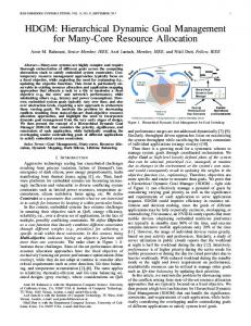
Figure 5: An example showing the effectiveness of application-level scheduling. In this section we begin with a motivation example, showing the potential effectiveness of application type scheduling, as shown in Figure 5. Let us consider a system in which there are two application types A1 and A2. The SP can accurately predict the generation time of the next service request. When the SP finishes processing requests and enters the idle state, it will go to sleep as long as the time until the next request is generated is more than . Otherwise it will remain in the idle state waiting for the next request. The SP wakes up from the sleep state as soon as a service request is generated. Two execution sequences have been considered. In the first sequence, there is no application scheduling. Each application is alternatively executed for exactly one unit of time. In the second sequence, we perform application scheduling that as long as one service request of application type A1 has been generated and serviced (note that the SP becomes idle at this time), we switch to application type A2, and we switch back to A1 when the second request of application type A2 has been generated and serviced. As shown in Figure 5, typically the service time for a request in the SP (e.g., HDD, WLAN card) is much shorter than the time taken in transitioning to and from the sleep state. It can be observed that the service requests are “grouped together” when using application-level scheduling, and thus both the power efficiency and performance are improved (i.e., the component sleeping time is maximized.) The applicationlevel scheduling technique used in Figure 5 (b), in which application type switch can happen only when the component is in the idle state, coincides with the CPU scheduling constraint stated in Section 4.2 that application type switch can only occur at idle-state decision epochs of the RL algorithm. It is validated using real traces that the application-level scheduling technique can improve both the
power efficiency and performance by reducing the number of transitions to and from the sleep state. We also consider the fairness issues among different types of applications in the application scheduling algorithm, which could satisfy the requirement of allocating a fair share of CPU execution time for each type of application. More formally, we impose a fairness constraint among different types of applications as follows. We use to denote the whole application type pool. For the ith ( ) type of application, we use to denote the total CPU occupying time of such type of application starting from time (i.e., the system starting time) until the current time . The fairness constraint states that each ith ( ) type of application cannot, on average, occupy more than percentage of the total CPU execution time, i.e., (9) Algorithm 1 presents the proposed CPU scheduling algorithm considering the fairness issue among different types of applications. In the proposed algorithm each ith ( ) type of application maintains and updates a value . Suppose that we are currently at subdecision epoch (which implies that the ith type of application is currently running in the CPU.) Recall that application type switch can only occur at the idle-state subdecision epochs. Then the proposed scheduling algorithm goes as follows: Algorithm 1: The CPU Scheduling Algorithm Considering the Fairness Issue. At the sub-decision epoch
: ( ) denotes the delta kronecker function.
, in which If
: If ( ) (in which is a predefined threshold value for CPU execution time): Find application type
with the minimum
value. Perform application type switch from type to type . Then we arrive at sub-decision epoch , with , assuming that the most recent subdecision epoch of application type is . End End If no application type switch happens, we arrive at subdecision epoch .
5. Experimental Results We present simulation results with the hierarchical DPM algorithm on a wireless adapter card (WLAN) card. Table 1 lists the power and delay characteristics of that device. In this table is the time taken in transitioning to and from the sleep state while is the energy consumption in waking up the device. refers to the break even time.
Table 1: Power and delay characteristics of WLAN card. 1.6 W 1.2 W 0.90 W *The WLAN card is turned off.
0 W*
0.9 J
0.3 s
0.7 s
For the baseline systems we use the RL-based DPM [9], as well as the expert-based DPM [7]. Three policies are adopted as experts in the expert-based DPM: fixed timeout policy, adaptive timeout policy, and exponential predictive policy [3], as shown in Table 2. Table 2: Characteristics of the expert-based policy. Expert Fixed Timeout Adaptive Timeout Exponential Predictive
Characteristics Timeout = any value Initial Timeout = , adjustment = ±0.1 ,
For the WLAN card, we have measured several real traces using the tcpdump utility in Linux, including a 45minute trace for online video watching, a 2-hour trace for web surfing, and a 6-hour trace for a combination of web surfing, online chatting and server accessing. The correct prediction rates of the Bayesian predictor are 99.2% for the video trace, 79.8% for the web trace, and 82.8% for the combined trace. We first compare the effectiveness of the proposed LPM (without considering the application-level scheduling issues) with the baseline DPM algorithms [7][9]. We conduct simulation using only one type of application with service request trace given by the 6-hour combined trace, similar to the experimental setups in the reference works [7][9]. Figure 6 gives the power and latency tradeoff curves achieved by the proposed LPM, the RL-based DPM proposed in [9], as well as three different expert-based DPM algorithms. The timeout values of the fixed timeout expert in those three algorithms are set to be , , and , respectively. We can see from Figure 6 that the proposed RL-based LPM method has a wider power-latency tradeoff range, especially when compared with the expert-based DPM algorithm. Even with the same latency, the proposed RL-based LPM achieves lower power consumption than the baseline algorithms (both the RL-based DPM algorithm and the expert-based DPM algorithm.) The improvement of the proposed RL-based LPM over the baseline RL-based DPM method proposed in [9] is mainly on state and action spaces, when only one type of application is running in the CPU. We further compare the effectiveness of the proposed RL-based hierarchical DPM framework with baseline DPM algorithms when multiple types of applications can run in the embedded system. We consider two types of applications, with service request traces given by the combined trace and the web surfing trace (we duplicate this trace so that it becomes a 4-hour trace), respectively. We name them the 1st and the 2nd types of applications, respectively. The ratio of the total CPU occupying time of these two types of applications should be 3:2. In the baseline systems, we use a simple application type switch technique, in which we switch from the 1st type to the 2nd type of application after the 1st type of application running in the CPU for 1 s, and we switch back after 0.67 s. Besides, the DPM algorithms in the baseline systems are ignorant of the application type information. In the proposed RL-based
hierarchical DPM framework, we can use one user-defined parameter to control the power-latency tradeoff for each type of application, independent of the other type of. In contrast, we can only control the power-latency tradeoffs of the two types of applications together in the baseline systems, without the ability of controlling them separately. Figure 7 gives the overall power and latency tradeoff curves achieved by the proposed hierarchical DPM framework, as well as the baseline systems. We can see from Figure 7 that the proposed hierarchical DPM framework consistently outperforms baseline systems. The maximum power saving with the same average latency is 31.1%, while the maximum amount of latency reduction without any power consumption increase is up to 41.8%, compared with the baseline systems. The Pareto superior performance of the hierarchical DPM framework compared with baseline systems is mainly due to (i) the more robust LPM specifically optimized for handling multiple types of applications, and (ii) the exploitation of the potential benefit of application-level scheduling.
for exploiting the potentially significant benefit of performing application-level scheduling on the component power optimization. In the hierarchical DPM framework, power and latency tradeoffs of each type of application can be precisely controlled based on a user-defined parameter. Experimental results demonstrate that the proposed hierarchical DPM framework achieves an evenly distributed power and latency tradeoff curve, which is Pareto superior to the power and latency tradeoff curves achieved by baseline DPM algorithms.
7. References [1]
[2]
[3]
[4]
[5]
[6]
[7] Figure 6: Comparison between the power-latency tradeoff curves of the 1st type of application (the combined trace.)
[8]
[9]
[10]
[11]
[12] Figure 7: Comparison between overall power-latency tradeoff curves of the two types of applications.
[13]
6. Conclusion
[14]
In this paper an architecture for hierarchical DPM to facilitate component power minimization in an embedded system has been proposed. The proposed (online) adaptive hierarchical DPM framework consists of (i) a componentlevel LPM which adopts model-free RL to effectively cope with variations and uncertainties emanated from hardware and application characteristics, and (ii) a system-level GPM
[15] [16]
L. Benini, A. Bogliolo, and G. De Micheli, “A survey of design techniques for system level dynamic power management,” IEEE Trans. on VLSI Systems, 2000. M. Srivastava, A. Chandrakasan, and R. Brodersen, “Predictive system shutdown and other architectural techniques for energy efficient programmable computation,” IEEE Trans. on VLSI, 1996. C. H. Hwang and A. C. Wu, “A predictive system shutdown method for energy saving of event-driven computation,” in ICCAD ’97. L. Benini, G. Paleologo, A. Bogliolo, and G. De Micheli, “Policy optimization for dynamic power management,” IEEE Trans. on CAD, Vol. 18, pp. 813833, Jun. 1999. Q. Qiu and M. Pedram, “Dynamic power management based on continuous-time Markov decision process,” in DAC ’99. T. Simunic, L. Benini, P. Glynn, and G. De Micheli, “Event-driven power management,” IEEE Trans. on CAD, 2001. G. Dhiman and T. Simunic Rosing, “Dynamic power management using machine learning,” in ICCAD ’06, pp. 747-754, Nov. 2006. Y. Tan, W. Liu, and Q. Qiu, “Adaptive power management using reinforcement learning,” in ICCAD ’09, pp. 461-467, Nov. 2009. Y. Wang, Q. Xie, A. Ammari, and M. Pedram, “Deriving a near-optimal power management policy using model-free reinforcement learning and Bayesian classification,” in DAC ’11, pp. 875-878, Jun. 2011. Y-H. Lu, L. Benini, and G. De Micheli, “Power-aware operating systems for interactive systems,” IEEE Trans. VLSI System, Apr. 2002. P. Rong and M. Pedram, “Hierarchical power management with application to scheduling,” in ISLPED ’05, pp. 269-274, Aug. 2005. Z. Ren, B. H. Krogh, and R. Marculescu, “Hierarchical adaptive dynamic power management,” DATE ’03. T. Simunic and S. Boyd, “Managing power consumption in networks on chips,” in DATE ’02. S. Bradtke and M. Duff, “Reinforcement learning methods for continuous-time Markov decision problems,” in Advances in Neural Information Processing Systems 7, pp. 393-400, MIT Press, 1995. R. S. Sutton and A. G. Barto, Reinforcement Learning: An Introduction, MIT Press, Cambridge, MA, 1998. C. M. Bishop, Pattern Recognition and Machine Learning, Springer, August 2006.