WM-78
1
Hierarchical OLSR – A Scalable Proactive Routing Protocol for Heterogeneous Ad Hoc Networks Ying Ge, Louise Lamont, Luis Villasenor
Abstract— The IETF’s mobile Ad Hoc networks (MANET) working group has designated the optimized link state routing (OLSR) as being one of four base routing protocols for use in ad hoc networks. Ad hoc routing protocols in general, including OLSR, do not scale well in heterogeneous networks, as they do not differentiate between the transmission capabilities of various member nodes, nor the channel access control scheme used by nodes when performing routing computations, even though many of the protocols support nodes having multiple interfaces. Under OLSR, for example, the control messages are sent to all interfaces, generating a very high overhead. In this paper, we propose optimizations to OLSR in order to limit the amount of control traffic generated and to make more efficient use of the higher capacity links found in heterogeneous wireless networks. Using OPNET simulations, we introduce a hierarchical mechanism to OLSR, and demonstrate that the Hierarchical OLSR (HOLSR) greatly reduces the required protocol overhead, which improves protocol scalability in large size heterogeneous networks. To our knowledge, this paper represents the first attempt made to address in-dept scalability issues of the OLSR protocol on heterogeneous wireless ad hoc networks. Index Terms— Wireless Networking, Mobile Ad Hoc routing, hierarchical protocol, scalability, OLSR.
I. INTRODUCTION
A
mobile ad hoc network (MANET) [1] is a dynamic multi-hop wireless network established by a group of mobile nodes on a shared wireless channel. Such a network may be self-contained, or it may be subsumed under a larger network. However, because member nodes are capable of random (individual) movement, network topology can change rapidly and unpredictably. Compared to a fixed-network architecture, an ad hoc network promises great advantages, Manuscript received January 7, 2005. This work is funded by Defense R&D Canada. Louise Lamont is with the Communications Research Centre, Government of Canada, 3701 Carling Av., Ottawa, Canada (phone: 613-991-9635; fax: 613-998-9648; email:
[email protected]). Ying Ge is with the Communications Research Centre, (email:
[email protected]). Luis Villasenor is with the CICESE Research Centre, Mexico (email:
[email protected])
such as the ability to instantly deploy mobile nodes, and the mobile nodes’ ability of reconfiguring and of preserving connectivity during topology changes. These features of ad hoc networks offer several interesting areas of study. Many contemporary ad hoc wireless networks are heterogeneous, being comprised of mobile devices equipped with interfaces having distinct communications capabilities with respect to data rate, radio range, frequency band, battery life, etc. In military networks for instance, soldiers, tanks and command posts might each be given wireless communications equipment appropriate to their level of communication. Rescue operations provide another case-in-point: individual rescuers usually are equipped with wireless communications devices powered by limited resources, which afford only limited transmission coverage and communications bandwidth; ambulances or police vehicles are outfitted with more powerful equipment providing extended communications coverage with higher communications bandwidth capability, enabling communication among vehicles; helicopters, as backbone of the rescue team, are equipped with additional interfaces providing direct point-topoint wireless communications with other helicopters, using carrier frequencies distinct from those of the ground radio network. Scalability is one of the most important factors governing the efficacy of heterogeneous wireless networks. Scalability may be defined as the ability of a network to adjust or maintain its performance when its size increases (and the demands made upon it become greater and greater). Yet under the existing “flat” routing protocol, the performance of an ad hoc network tends to degrade as the number of mobile nodes increases, because a flat routing protocol cannot differentiate the capacities of its member nodes, and does not scale well for typical heterogeneous networks of the type just described. Furthermore, when the flat routing protocol is used, the resulting control overhead may be doubled or even tripled, depending on the number of interfaces possessed by the nodes. More importantly, the high-capacity links are not efficiently exploited under such a routing strategy. In this paper, we present an approach specifically designed to improve the scalability of the Optimized Link State Routing protocol (OLSR) [2], rendering it more suitable as a routing protocol for large-scale heterogeneous communications
WM-78
2
networks. Our work differs from existing literature on the hierarchical routing of heterogeneous networks (such as [3], [4], [5] and [6]) in that the hierarchical scheme here presented is fully integrated within the OLSR protocol, so it does not require any additional network layer protocols or algorithms. The hierarchical network architecture consists of multiple ad hoc networks dynamically formed at distinct logical levels in the network topology, and is not restricted to any particular addressing scheme. We make use of the different components in the heterogeneous network while organizing the hierarchical structure dynamically. With this hierarchical structure we propose optimizations to OLSR in order to reduce message overhead and routing-table size of nodes limited by low processing power, and to make more efficient use of the higher capacity links in the network. Furthermore, the hierarchical structure releases the OLSR from having to perform frequent routing computations, as the local movement of member nodes is now handled within the cluster, without affecting other parts of the network. Using OPNET [7] simulations, we demonstrate that the Hierarchical OLSR (HOLSR) does scale more efficiently: overhead is dramatically reduced, and protocol performance is greatly improved with respect to “packet delivery ratio” and “end-to-end delay”. With the hierarchical approach, we not only retain the advantage of a proactive routing protocol – the connection setup delay is minimized – but also improve two aspects of the protocol: 1) heavy overhead is reduced and 2) frequent route updates are avoided. Thus, for large heterogeneous wireless networks, HOLSR yields very promising results as compared to those achieved by the original (flat) OLSR protocol. The remainder of this paper is organized as follows: Section 2 gives an overview of OLSR and introduces the proposed hierarchical mechanism; Section 3 covers the OPNET simulation environment; Section 4 compares the results, obtained via OPNET simulations, of the HOLSR versus the flat OLSR protocols in the areas of control overhead, computational overhead and protocol performance; Section 5 highlights the main contributions of this work. II. OLSR AND HOLSR A. OLSR The OLSR protocol is a proactive routing protocol for mobile ad hoc networks. It optimizes the pure link state protocol by propagating the topology information via selected nodes, which are called multipoint relays (MPRs). In the OLSR protocol, two types of control messages are used for topology information: the Hello message and Topology Control (TC) message. A node sends a Hello message to identify itself and to report a list of neighboring mobile nodes. From a Hello message, the mobile node receives information about its immediate neighbors and 2-hop neighbors, and selects MPRs accordingly (for details of the MPR selection mechanism, please refer to [2]). A TC message originates at an MPR node announcing who has selected it as
an MPR. Such messages are relayed by other MPRs throughout the entire network, enabling the remote nodes to discover the links between an MPR and its selectors. Based on such information, the routing table is calculated using the shortest-path algorithm [8]. The OLSR supports nodes having multiple interfaces. A "flat" mechanism is employed, whereby a node sends Hello and TC messages through all its interfaces without regard to the link capacities of the other nodes, and references to nodes of differing transmission capabilities are grouped together in the Hello and TC messages. The HOLSR, however, uses a different strategy when propagating Hello and TC messages, which is discussed in detail in the following sub-Section. B. HOLSR The HOLSR model is based on the protocol specifications for the OLSR algorithm. HOLSR dynamically organizes nodes into cluster levels. The cluster structure supports random movement of the nodes and has diagnostic capabilities. The main improvements realized by the HOLSR protocol are a reduction in the amount of topology control information needing to be exchanged at different levels of the hierarchical network topology, and the efficient use of high capacity nodes. Another significant benefit is a reduction in routing computational cost: if a link in one part of the network is broken, only those nodes within that cluster need to recalculate the routing table, while nodes in other clusters are not affected. More importantly, HOLSR is versatile in that it does not require a logical addressing scheme but can accommodate one if required. B.1- HOLSR Logical Topology Levels The proposed network architecture for the HOLSR is illustrated in Fig 1. Based on the different components in the network, the nodes are organized into multiple logical topology levels. The low-power nodes, designated by circles, are equipped with only one interface offering limited data rate and transmission range. Such nodes participate at the topology Level 1, and can represent rescue personnel whose communications are constrained by the limitations of the communications equipment these individuals can carry. Nodes at the topology Level 2, designated by rectangles, are equipped with two interfaces, one of which is a wireless interface capable of communicating with Level 1 nodes. These mobile nodes can also relay messages at the logical topology Level 2 using a frequency-band or a medium-access control (MAC) protocol which differs from the one used for communication at the topology Level 1 – this additional wireless interface affords a longer transmission range than the one used by Level 1 nodes. Such nodes can represent mobile units such as ambulances and police forces, capable of communicating with individual personnel as well as with other mobile units on different frequency bands. Topology Level 3 nodes, designated by triangles, can represent helicopters. These nodes are equipped with three
WM-78 wireless interfaces capable of communicating in turn with Level 1 and Level 2 nodes and with other Level 3 nodes via high-speed point-to-point direct wireless links.
Fig.1. An example of a heterogeneous network
At each logical topology level, nodes form clusters, select MPRs, and exchange network topology information independently. Unlike the original (flat) OLSR, which transmits the same topology control information from all interfaces [2], in HOLSR each interface sends out topology information relating only to its own level. In actuality these interfaces run HOLSR independently as individual nodes. The elements in Fig.1 are designated as follows: Clusters are labeled by an uppercase 'C' (denoting 'Cluster'), followed by a digit indicating the topology Level at which the cluster is grouped, followed in turn by an uppercase letter indicating which node functions as cluster head. Thus for example, C2.B designates a Level 2 cluster having node B as cluster head, etc. Nodes are designated in one of two ways, depending on whether they are single-interface or multiple-interface nodes, as follows: Nodes indicated by small CIRCLES possess only one interface, and each such node is represented by a single digit (1, 2, 3, etc.); these nodes are found only at the bottom Level. Multiple-interface nodes, which operate on multiple topology Levels, are represented by two characters: an uppercase letter designating the node's name (A, B, C, etc.) followed by a digit indicating the node's interface, the digit corresponding to the topology Level at which that interface operates. Nodes with interfaces indicated by TRIANGLES can operate at each of the three Levels (viz: B3, B2, B1), while nodes with interfaces indicated by SQUARES operate at only the lower two Levels (viz: E2, E1). Please note: in reality, nodes do not always follow strictly the interface guidelines outlined above. For instance, topology Level 3 nodes could conceivably possess only two interfaces: one to communicate with peers in Level 3, and the second to communicate with nodes in Level 2 below. This is exemplified by node F in our illustration, which is a Level 3 node possessing only two interfaces.
3 B.2- HOLSR Cluster Formation Mobile nodes form different cluster levels, a cluster being comprised of a group of mobile nodes (at the same topology level) having selected a common cluster head. Clusters are self-organized, with cluster heads being configured during the start-up of the HOLSR process, whereby any node participating in multiple topology levels automatically becomes the cluster head of any lower-level nodes. In the above example, node A, which participates in both topology Levels 1 and 2, can become the Level 1 cluster head, while B, which participates in topology Levels 1, 2 and 3, can become the cluster head at both Level 1 and Level 2. At each level the cluster head declares its status and invites other nodes to join its cluster by periodically sending out Cluster ID Announcement (CIA) messages (these are sent together with the Hello messages to reduce the number of packet transmissions). CIA messages contain two fields: cluster head, which identifies the interface address of the cluster head selected by the message generator, and distance (in hops) to that cluster head. When a cluster head generates a CIA message, it identifies itself within the cluster head field, with distance being 0. The nodes in proximity to the cluster head receive the CIA messages, join the cluster, and begin generating CIA messages inviting nodes further away to join the cluster. Any given node may receive two or more CIA messages, indicating that it is located in the overlapping regions of several clusters. In such cases, the node joins whichever cluster is closest in terms of the hop count. For instance, in our example interface A1 of node A sends out the following CIA message: “cluster head: A1; hop count: 0”. The CIA message is received by A1’s next-hop neighbor, node 1, who then joins cluster C1.A and generates a CIA message: “cluster head: A1; hop count: 1”, which is received by node 2. Therefore, node 2 also joins cluster C1.A. Node 3, which is in the transmission range of both 2 and B1, receives two CIA messages: one from 2 indicating: “cluster head: A1; hop count: 2”, and one from B1 indicating: “cluster head: B1; hop count: 0”. In this case, node 3 chooses to join the closer cluster C1.B, managed by B1. Following this process, each Level 1 node joins a selected cluster, and the mechanism is in turn applied at each respective topology level. It should be noted that given the random movement of the mobile nodes, a node might find a cluster head that is closer than the one to which it is currently attached. In this case, the mobile node will proceed to change its cluster and attach itself to the closest cluster head. A built-in diagnostic feature helps ensure the robustness of HOLSR's clustering mechanism: as CIA messages are generated, each node monitors the time-out value of the CIA messages received. Should a cluster head become inactive or move away, no CIA message is received after a period of time and the original CIA information becomes invalid. The node can then accept a CIA message from another cluster and will join that cluster should the opportunity present itself. As per our example, suppose B1 goes down; after B1’s CIA has
WM-78 timed out, 3 can join cluster C1.A when it receives the CIA message from 2; 5 joins cluster C1.C upon receiving the CIA message from 6; finally, 4 also joins cluster C1.C when receiving the CIA message from 5, after 5 has joined C1.C. The clusters are therefore automatically reconfigured. If no CIA messages are received, that is, if the network is no longer heterogeneous and is comprised of nodes having only a single interface (i.e., there are no longer any multiple-interface nodes in the network), the HOLSR treats the entire network as one cluster, and behaves as would the original OLSR. B.3- HOLSR Cluster Head Message Exchange In HOLSR, a cluster head acts as gateway through which messages from cluster members are relayed to other parts of the network; therefore each cluster head needs to be aware of the membership information of its peer cluster heads. A Hierarchical TC (HTC) message is used to transmit the membership information of a cluster to the higher hierarchical level nodes. Three basic types of HTC messages are used: the full membership HTC message, the update HTC message and the request HTC message. The full membership HTC messages are periodically transmitted by a cluster head to provide information about its cluster members, including members of any lower-level clusters beneath it. The update HTC messages provide information with respect to cluster membership changes, that is, the update HTC messages are used when mobile nodes join or leave a cluster. As HTC messages carry a sequence number field, it is possible to determine whether any HTC packet loss has occurred, in which case a request for the re-transmission of a full membership HTC message is sent by the receiving node. HTC forwarding is enabled by MPRs, and is restricted within a cluster. As per our example, node A, which is the cluster head of Cluster C1.A, generates HTC messages from interface A2 informing other Level 2 nodes that 1, 2 and A1 (itself in Level 1) are members of its cluster. B, which is the cluster head of Cluster C2.B, generates HTC at topology Level 3, advertising that 1,2,3,4,5,A1,B1 (at topology Level 1) and A2,B2 (at topology Level 2) are members of its cluster. A’s Level 2 HTC is relayed to other Level 2 nodes within Cluster C2.B; B’s Level 3 HTC is relayed to other Level 3 nodes. In topological terms, the higher a given node is located, the more information it obtains about the network. Nodes at the highest topology level possess full knowledge of all nodes in the network, consequently the sizes of their routing tables are as large as they would be under OLSR. However, because the topology information required by lower-level nodes is limited in scope, the sizes of their routing tables are consequently reduced as compared to the original (flat) OLSR.
4 level, TC messages are generated independently. The propagation of the TC is usually restricted within a cluster, unless a node is located in the overlapping regions of several clusters. For example, 2 in Cluster C1.A may accept a TC from 3, which is in Cluster C1.B, and forward it to 1. However, 1 retains only the information relating to that TC, without passing it on. Therefore, an HOLSR node's location directly determines the required scope of its knowledge of network topology: for nodes located towards the center of the cluster, TC propagation is limited to the local cluster; for nodes located in the overlapping regions of multiple clusters, the TC message is propagated not only within the local cluster but to neighboring clusters as well. This approach offers two main advantages: 1) the control message reflecting local movement is restricted within the local area, which largely reduces protocol overhead as well as routing-table computation overhead; 2) nearby nodes in different clusters at the same level can communicate directly without having to follow the strict clustering hierarchy, which decreases delay and reduces the load on the cluster head. B.5- Data Transfer using the Clusters For data transmissions outside the local area, the gateway mechanism employed can be illustrated as follows: 1, which is a member of Cluster C1.A, intends to send data to 10, which is in Cluster C1.E. From Hello and TC messages, 1 knows that 10 is not a member of its cluster, so it sends data to its cluster head A. A in turn does not recognize 10 as a member of its cluster, nor does it see 10 from the TC or HTC messages (which convey only the topology or membership information within Cluster C2.B), therefore A relays the data packet to its cluster head B. B in turn knows from the HTC message originated by F (which is within its Level 3 cluster) that 10 is a member of F’s cluster, therefore the data packet is relayed to F, and finally to its intended destination 10 via E (which is the head of the cluster where 10 locates). As we trace the transmission route traveled by the data packet (1Æ A Æ B Æ F Æ EÆ10), we see that the cluster head is always used as the gateway by member nodes at lower hierarchical levels when transmitting to destinations outside the local area. However, when data is transmitted between neighboring nodes, the cluster head is not involved even through the nodes may belong to different clusters. In the case of node 2 (member of cluster C1.A) transmitting data to B1 (member of cluster C1.B), the data packet is directly relayed to B1 through 3, as 2 knows that it can reach B1 via 3 from 3’s TC (see the above discussion outlining how a node accepts the TC from other clusters.) With this strategy the HOLSR makes efficient use of high capacity nodes without overloading them.
B.4- HOLSR Topology Control (TC) Propagation
C. HOLSR for Group Movement
Nodes at each hierarchical level independently select MPRs in their respective cluster level: in the above example, nodes in Cluster C1.A select MPRs at Level 1, while nodes in Cluster C2.B select MPRs at Level 2. At each hierarchical
HOLSR clustering does not require a logical hierarchical address scheme (as discussed in [9]), but one can be employed if desired, as might be the case in situations where a network exhibits group mobility (for instance when foot soldiers and
WM-78
5
vehicles move together in the field). In such cases all members of the group are assigned the same subnet address, representing that group. In our example above, node 1’s IP address 192.168.2.1 can be read as follows: 192 indicates node 1 is within Cluster C3.B at topology Level 3, 168 represents Cluster C2.B at Level 2, 2 means Level 1 Cluster C1.A, 1 is the node itself. When an HOLSR node broadcasts a HTC message, it need only broadcast its cluster address at the local topology level, without having to broadcast the addresses of all its cluster members. We assume that the pool of valid node addresses is known in advance, which precludes nodes from attempting to communicate with a non-existing node. If a node has become unreachable, eg. a soldier’s communication equipment has become non-operational, the cluster head can simply use the update HTC to specify that the node in question is no longer available. Hence the HTC size is greatly reduced, further reducing the HOLSR message overhead. The sizes of the routing tables of the higher-level nodes are also reduced because the routes to all nodes in a remote cluster can be represented via a single subnet address entry. III. OPNET SIMULATION SCENARIO The OPNET [7] simulation tool is used to evaluate and compare the performances of the HOLSR and the flat OLSR. The general layout of a heterogeneous network is simulated: two subnets are connected to each other via a point-to-point trunk. Each subnet occupies a 1200m x 1200m flat space, and contains several types of mobile nodes detailed as follows (802.11b was chosen as the physical layer used by all the mobile nodes. Also, we assume that because of the high power-levels used by nodes at Levels 2 and 3, the range of the those nodes' 802.11b interfaces is extended when operating with higher data rates. Also, we assume that that the frequency band of the interfaces are carefully selected so that an increase of the transmission power will not cause interference with other interfaces): • 45 Level 1 nodes – Level 1 nodes are equipped with the least powerful equipment: a wireless card having a data rate of 1Mbps and a transmission range of 250m. • 15 Level 2 nodes – Each Level 2 node is fitted with two wireless cards: one card is identical to that carried by the Level 1 nodes; the other card supports a data rate of 5.5Mbps and a transmission range of 750m, using a frequency band different from that of the Level 1 nodes. • 5 Level 3 nodes – The Level 3 nodes are the backbone of the wireless subnet. In addition to the interfaces used by the Level 2 nodes, Level 3 nodes are equipped also with another wireless-interface card operating on a distinct carrier frequency and supporting point-to-point wireless communications at the highest available data rate of 11Mbps. Although the above description outlines the concept of “topology level” as used in HOLSR, in our simulation the flat OLSR nodes were likewise equipped with the same (multiple)
interfaces, because OLSR also supports nodes having multiple interfaces. The node movement considered in this paper is that of random (individual) movement rather than that of group movement. The Level 1,2,3 nodes each operate within a “maximum speed”, as follows: Level 1 node = 3m/s (10.8km/h); Level 2 node = 10m/s (36km/h); Level 3 node = 0m/s (Level 3 nodes are always inter-connected via point-topoint wireless links). Each mobile node changes its location within the subnet based on the “random waypoint” model [10], that is, the node randomly selects a destination, moves towards that destination at a speed not exceeding the maximum speed for that level, and then pauses – this interval being known as pause-time. In order to calculate the effect of node movement on the protocol overhead and performance, four distinct pause-time values are given in the simulations: 0s (continuous movement), 150s, 300s, 600s (no movement) in a 600 second simulation time. IV. OPNET SIMULATION RESULTS In this section, the control overhead, computational overhead and protocol performance of the flat OLSR and the HOLSR are compared and analyzed. As OLSR supports nodes having multiple interfaces, both OLSR and HOLSR were run under the scenario discussed in Section III. Data was collected via multiple runs of OPNET simulation. “Control Overhead” – a measure of the number of OLSR packets transmitted. An individual OLSR packet may contain one or more OLSR messages: Hello (in HOLSR, the CIA and Hello are sent out in one packet), TC, and HTC (in HOLSR), etc. Table I gives the average number of OLSR packets generated or relayed in the network for each of the five pausetime values. TABLE I COMPARISON OF NUMBER OF PACKETS TRANSMITTED (PACKETS/S) Pause Time HOLSR Flat OLSR
0s 420 2697
150s 422 2946
300s 420 2705
600s 416 2615
As Table I demonstrates, HOLSR significantly reduces topology control overhead in comparison with the flat OLSR. This is because the flat structure of the OLSR necessitates that topology control messages transmitted by a multiple-interface node be sent through all interfaces possessed by that node[2], greatly increasing the number of TC messages transmitted in a network where many nodes possess multiple interfaces. By contrast, HOLSR achieves its reduction of overhead because the nodes in the network are grouped into distinct hierarchical clusters, and the propagation of topology control messages is limited within the local area, which prevents these messages from flooding the entire network, while message flooding through multiple interfaces is also avoided, because only the interface related to the topology level of the message is used. “Computational Overhead” – the total number of routing
WM-78
6
table calculations performed in one second; the data is collected only for continuous movement (parsing time 0), this being the worst-case scenario where the largest number of routing-table updates are introduced. TABLE II COMPUTATIONAL OVERHEAD HOLSR Flat OLSR
100 2700
Table II shows the average computational overhead for the HOLSR and the OLSR protocols. From these results it is clear that the HOLSR protocol achieves a substantial reduction in the computational overhead. This reduction in HOLSR is realized as the topology updates are handled locally in each cluster, as opposed to OLSR in which topology updates are propagated thru the entire network. “Protocol Performance” – this is evaluated using two metrics: “Packet Delivery Ratio” and “End-to-End Delay”. We use three types of UDP traffic patterns to observe the protocol performance under different network traffic conditions. Light traffic, medium traffic, and heavy traffic patterns are shown in the following table:
Traffic Pattern
TABLE III TRAFFIC PATTERN Communication Data Pairs Size (bytes)
delivers at least 20% more packets under all network traffic patterns. Based on our discussion of control overhead, such improvements result from the low overhead incurred by HOLSR. As per our simulation, it can be observed that the excessive overhead generated by the flat OLSR engenders a large number of collisions of the control packets, which contain network topology information. When these packets are lost, the IP routing tables cannot be correctly updated. Consequently, many data packets cannot be delivered to their intended destination because of incorrect IP routing table entries. In addition, many data packets possessing the correct route may also be dropped as a result of data congestion in the wireless media and this is especially true under heavy network traffic. • End-to-End Delay: the average elapsed time between transmission and reception of individual data packets Fig. 3. compares the end-to-end delays of the two versions of OLSR protocols.
Number of Packets sent Second for Each Communication Pairs
Light Traffic
40
64
4
Medium Traffic
30
256
4
Heavy Traffic
30
512
4
• Packet Delivery Ratio: percentage of data packets successfully delivered to the receiver nodes against total packets sent. Fig. 2. gives the packet delivery ratios for both HOLSR and flat OLSR for the 3 traffic patterns.
Fig. 2. Comparison of “packet delivery ratio”
Compared with the flat OLSR, the packet delivery ratio achieved by HOLSR is much higher: on average, the HOLSR
Fig. 3. Comparison of “end-to-end delay”
Under light and medium network traffic, HOLSR delivers data packets more quickly and efficiently than does the flat OLSR because under HOLSR the generated overhead is much lower. Reduced traffic in the wireless media allows the HOLSR to realize a shorter queuing delay, resulting in shorter end-to-end delays. Also, the HOLSR groups nodes into different cluster levels, whereby those nodes equipped with multiple interfaces become cluster heads. These cluster heads employ higher data-rate wireless interfaces, acting as the “backbone” for the data packet transfers between different clusters. Thus, unlike with the flat OLSR, HOLSR capitalizes on the higher-capacity wireless media for data transmission and is thus more efficient in data packet delivery. Under heavy network traffic, HOLSR’s end-to-end delay is larger than that of the flat OLSR. This is due to the high overhead generated by the flat OLSR. The data packets that have to travel longer distances have a higher probability of getting dropped. The delay measurements will reflect mostly the data packets that have gone through fewer hops, hence the shorter end-to-end delay.
WM-78
7 V. CONCLUSION
REFERENCES
In this paper, we proposed an efficient approach for dynamically incorporating a hierarchical structure into the OLSR protocol in order to improve the OLSR’s scalability in heterogeneous networks where nodes move randomly. We have seen that implementation of this hierarchical mechanism not only reduces message overhead and routing table size, but that the frequency of routing updates is also reduced. Results of our heterogeneous network simulation confirm that, in comparison with the original OLSR, the HOLSR dramatically reduces protocol overhead within the network, achieves a higher packet-delivery ratio while incurring shorter queuing delays and shorter end-to-end delays, and reduces or eliminates the incidence of lost packets resulting from high overheads. HOLSR thus successfully and significantly improves the scalability of the original OLSR protocol in a heterogeneous network environment.
[1] J. Macker, S. Corsen, IETF Mobile Ad Hoc Networks (MANET) Working Group Charter, http://www.ietf.org/html.charters/manet-charter.html
ACKNOWLEDGMENTS This work was funded by Defence Research and Development Canada (DRDC). The authors would like to thank Darcy Boucher for his contributions on this paper.
[2] T. Clausen, P. Jacquet, et. al.; “Optimized link state routing protocol,” RFC 3626; http://www.faqs.org/rfcs/rfc3626.html; October, 2003. [3] S. Zhao, K. Tepe, I. Seskar and D. Raychaudhuri, "Routing protocols for self-organizing hierarchical ad hoc wireless networks," IEEE Sarnoff Symposium, Trenton, NJ, March 2003. [4] D. L. Gu, G. Pei, H. Ly, M. Gerla, B.Zhang, X. Hong; “UAV aided intelligent routing for ad hoc wireless networks in single-area theater,” IEEE WCNC, pp.1220-1225,2000. [5] K.Xu and M.Gerla; “A heterogeneous routing protocol based on a new stable clustering scheme,” MILCOM’02; October 2002. [6] Kaixin Xu, Xiaoyan Hong, and Mario Gerla. “Landmark routing in ad hoc networks with mobile backbones,” Journal of Parallel and Distributed Computing, vol.63, issue 2, 2003, pp.110-122. [7] www.opnet.com [8] E.Dijkstra, “A note on two problems in connexion with graphs,” Numerische Mathematik, pp. 269-271,1959. [9] G.Pei, M.Gerla, X.Hong and C.-C.Chiang, “A wireless hierarchical routing protocol with group mobility,” IEEE WCNC’99, New Orleans, LA, September 1999. [10] David B. Johnson and David A. Maltz, “Dynamic source routing in ad hoc wireless networks,” In Mobile Computing, edited by Tomas Imielinski and Hank Korth, Chapter 5, pages 153-181, Kluwer Academic Publishers, ISBN: 0792396979, 1996.