The International Archives of the Photogrammetry, Remote Sensing and Spatial Information Sciences, Volume XLII-4/W8, 2018 FOSS4G 2018 – Academic Track, 29–31 August 2018, Dar es Salaam, Tanzania
HIERARCHICAL PATH PLANNING FOR WALKING (ALMOST) ANYWHERE K. Landmark∗, E. Messel Norwegian Defence Research Establishment (FFI), P.O. Box 25, 2027 Kjeller, Norway -
[email protected] Commission IV, WG IV/4 KEY WORDS: Path planning, Clustering algorithms, LiDAR, Terrain mapping, Graph theory, Cost function, Walking, Open data
ABSTRACT: Computerized path planning, not constrained to transportation networks, may be useful in a range of settings, from search and rescue to archaeology. This paper develops a method for general path planning intended to work across arbitrary distances and at the level of terrain detail afforded by aerial LiDAR scanning. Relevant information about terrain, trails, roads, and other infrastructure is encoded in a large directed graph. This basal graph is partitioned into strongly connected subgraphs such that the generalized diameter of each subgraphs is constrained by a set value, and with nominally as few subgraphs as possible. This is accomplished using the k-center algorithm adapted with heuristics suitable for large spatial graphs. A simplified graph results, with reduced (but known) position accuracy and complexity. Using a hierarchy of simplified graphs adapted to different length scales, and with careful selection of levels in the hierarchy based on geodesic distance, a shortest path search can be restricted to a small subset of the basal graph. The method is formulated using matrix-graph duality, suitable for linear algebra-oriented software. Extensive use is also made of public data, including LiDAR, as well as free and open software for geospatial data processing.
1. INTRODUCTION The Detailed National Elevation Model, Norway’s biggest land surveying project, will by 2022 provide an airborne laser scanning (LiDAR) dataset covering the entire country with 2–5 measurements per m2 (Kartverket [Norwegian Mapping Authority], 2018). Authorities are making the data freely and openly available to the public, and encourage their use in new worthwhile applications. Similar initiatives are found in, e.g., the UK, where the Environment Agency is carrying out LiDAR scanning of the entire country and publishing recorded data under an Open Government Licence via the data.gov.uk portal, the stated aim of which is transparency and innovation (Data.gov.uk, 2018). Such data, we believe, render possible general path planning and mobility analysis covering any part of a land area, not just transportation networks; its wide range of applications including archeology (Herzog, 2014), public transit planning, physical exercise and hiking, forestry, and search and rescue operations (Ciesa et al., 2014). In particular, LiDAR data are used to generate detailed digital terrain and surface models (DTMs and DSMs) from which terrain slope, surface roughness, and obstacles can be determined, information which is crucial for general path planning. In addition, land cover classification (e.g., tree species) using aerial LiDAR is currently an emerging field of research, and also provides important information for mobility analysis. Automated (computerized) path planning has become a standard navigational aid in GNSS1-equipped vehicles, and is a critical component in autonomous systems such as self-driving cars. Path planning in road networks is routinely solved using graph theory (Balakrishnan and Ranganathan, 2012). In a directed graph (digraph) with n nodes and m arcs representing road segments, Dijkstra’s algorithm (Dijkstra, 1959) finds a minimum-cost solution in running time O[m log n]. Exploiting the natural hierarchical structure of road networks, modern routing applications ∗Corresponding 1Global
author Navigation Satellite System
achieve query times orders of magnitude smaller (in large networks), see, e.g., (Delling et al., 2009), (Bast et al., 2007). Crosscountry movement presents new challenges; there is no natural hierarchy, and there are two degrees of freedom instead of one. This increases graph complexity and, consequently, the computational load; in two dimensions typically 4 ≤ m/n ≤ 8 with roughly uniform node density (nodes per unit area). Modeling cross-country movement is difficult also because mobility, speed, and efficiency depend highly on the nature of the terrain and the means of transport, and, moreover, because it is not necessarily obvious how the data (or which data) should be adapted in the model. This paper describes one approach to computing optimum paths that are not bound to transportation networks. This requires a regular or random graph that covers the entire land area, is connected to road and pathway networks, and takes into account terrain features, man-made or natural obstacles, and infrastructure in general. Although cross-country path planning is a many-faceted problem, we concentrate on three issues: 1) partitioning large, nearly regular, geographically embedded graphs, 2) using a hierarchy of simplified graphs to reduce computational complexity, and 3) obtaining a cost function for walking humans. The purpose is to provide brief but sufficient detail to understand the source code and main algorithms. In addition we report on the use of open source software and open data. All aspects of the general path planning problem can be implemented with a suite of FOSS4G tools, in particular, the processing of LiDAR (point cloud) data, adaptation of vector and raster geospatial data, graph representation and storage, and optimum route search. Algorithms for generating and partitioning graphs are formulated using the matrix representation of directed graphs, suitable for array-oriented software such as NumPy/scipy.sparse, Julia, or GNU Octave (also open source software) as well as MATLABQR and other linear algebra APIs. Section 2 describes the graph model underlying our routing solu-
This contribution has been peer-reviewed. https://doi.org/10.5194/isprs-archives-XLII-4-W8-109-2018 | © Authors 2018. CC BY 4.0 License.
109
The International Archives of the Photogrammetry, Remote Sensing and Spatial Information Sciences, Volume XLII-4/W8, 2018 FOSS4G 2018 – Academic Track, 29–31 August 2018, Dar es Salaam, Tanzania
tion. A sequence of graphs G = (G0, G1, . . . , GH−1) represents the same physical area with decreasing levels of detail. This requires a method for partitioning large graphs. Section 3 develops a cost function for humans on foot. The mechanics and energetics of walking are complex and not fully understood. Hence empirical results are required, some of which are summarized here. However, biomechanical principles can be used to constrain the relation between walking speed (or energy expenditure) and key parameters such as terrain slope. Section 4 is a brief summary of the data processing pipeline and preliminary routing service application, implemented with open source software. Details on the datasets on which the graph model is based are also provided. 2. METHOD 2.1 Matrix graph duality Formally we work with a simple, directed, weighted graph, G = (V, E, w), where V = { v1, v2, . . . , vN } is the set of nodes (or vertices), E is a set of unique ordered pairs (vi, vj ) of nodes (the arcs), where i /= j (no self-loops), and w : E → R is the weight function. The order of G is n(G) ≡ N . We refer to the subscript k as the node index of vk . Each node v has a spatial position, denoted x(v) ∈ R3, as well as other attributes described below. A simple graph has no parallel arcs and can be represented by a square N × N matrix G = (wij ) by setting ( w(a), if a ≡ (vi, vj ) for some arc a ∈ E wij ≡ G[i, j] = otherwise. 0, (1) The adjacency matrix AG = (cij ) is defined such that cij is the number of arcs incident out of vi and into vj. For a simple graph with positive weights, AG = [G > 0] (a logical/binary matrix).
(2)
In path planning applications N is large while each node is incident with only about 1–10 arcs, so G and AG are sparse. A set of R distinct nodes, { vk1 , vk2 , . . . , vkR }, can be identified with a binary column vector with unity in the kj th row for j = 1, 2, . . . , R. In particular, the node vk is a binary vector with unity only in the kth row, and its neighbors in the matrix representation are N (G, vk ) = ATGvk,
(3)
i.e., a sparse matrix-vector multiplication, where AGT denotes the transpose matrix. This is a breadth-first search (BFS) step (Kepner, 2011). 2.2 Subgraphs and index maps We frequently operate on subsets of G, and G itself will be constructed by assembling smaller graphs. For a subset of nodes 1 U = { vk1 , vk2 , . . . , vkR } ⊆ V , a particular subgraph G 1 is obtained by keeping all edges incident only with nodes in U : U 1 1 V (G 1 ) = U and E(G 1 ) = { (u, v) ∈ E(G) : u, v ∈ U }. (4) U U 1 The matrix representation of G 1 can be obtained as the sparse U matrix product GU = U T GU (5) where U = [ vk1 vk2 . . . vkR ] is a sparse, binary N × R matrix and U T is its transpose. We can also view this as an indexing
operation in array-based languages, i.e.,
where
GU = G(IG→U , IG→U )
(6)
IG→U ≡ [ k1 . . . kR ].
(7)
The operation (6) extracts rows k1, . . . , kR and likewise columns k1, . . . , kR from WG. In NumPy syntax, this would be written WG[numpy.ix (IG→U , IG→U )]. Note that in NumPy and Julia, this creates a view (SciPy, 2018) into the original matrix, so matrix values are not copied from the parent graph. 11 is independent of the order of elements in IG→U , and set opG U erations may be defined on index vectors. For two sets of nodes, Ua, Ub ⊆ V (G), we write IUa →G ∪ IUb →G = IUa ∪Ub →G, a concatenated vector with duplicate indices removed. Similarly, IUa →G ∩ IUb →G = IUa ∩Ub →G is a vector of common indices in Ua and Ub. Mapping between node indices in the subgraph and parent graph can be accomplished by defining a (normally sparse) 1 n(G) × 1 vector I− G←U with non-zero entries given by −1 IG←U (IG →U ) ≡ [ 1 2 . . . R ]. (8) 1 If J is a vector of node indices with respect to G 1 (so max J ≤ U R), then ) − IG→U I 1 (J ) = J. G←U
Conversely, if I is a vector of node indices with respect to G (so max I ≤ N ), then I−1 G←U (IG→U (I))
= I.
This construction can be nested. rIf 1H l1 ⊆ U ⊆ V (G), and J is a vector of indices with respect to G 1 1 , then the correspondU H ing indices with respect to G are ( \ I = IG→U I 11U →H (J ) , G
and so on. 2.3 Distance In a simple digraph, G, a path from node s to t is a sequence of distinct nodes P = (v1 = s, v2 , . . . , vR = t) in V (G) such that each consecutive pair (vi, vi+1) is in E(G). The length of P is ), |P | = R−1 w(v , vi+1), and the distance from s to t, denoted i i=1 dG(s, t), is the length of a minimum-length path from s to t. For a spatial graph there is also distance as a function of the two node positions, i.e., Euclidean or geodesic distance. We use Euclidean distance in an appropriate projected reference system, as it is fast and simple to compute, and denote it dEUCL. For the purpose of partitioning the graph (Section 2.5), we need a single-source distance-to-all-nodes algorithm, such as Dijkstra (if w > 0). However, with the clustering algorithm (Section 2.5) in mind, Dijkstra is modified in a heuristic manner, as in Function 1: once the set of closed nodes has expanded beyond a cutoff distance, Λ, the remaining active nodes are assigned the larger value of dEUCL/c and Λ, where c is a scaling factor. If the weight function is travel time, then c will be a characteristic speed value. As implemented in Function 1, c is determined from the graph locally, and may vary across the graph. Depending on the application, c could also be a preset global parameter to further speed up computation. The cut-off distance, Λ, is typically chosen to be a few times the characteristic cluster size of the desired graph partition (Section 2.5). Although shortest path algorithms can be
This contribution has been peer-reviewed. https://doi.org/10.5194/isprs-archives-XLII-4-W8-109-2018 | © Authors 2018. CC BY 4.0 License.
110
The International Archives of the Photogrammetry, Remote Sensing and Spatial Information Sciences, Volume XLII-4/W8, 2018 FOSS4G 2018 – Academic Track, 29–31 August 2018, Dar es Salaam, Tanzania
Function 1 Distance function (modified Dijkstra)
Function 2 Adjacency matrix, graph partition
Require: G, a finite, simple, positive-weight (w), spatial digraph Require: s ∈ V (G), the source node Require: Geographical distance function dEUCL : V × V → R Require: Λ > 0, cut-off distance
Require: G, a finite, simple digraph Require: L, label vector for partition of G
1: function DISTANCE(G,s,Λ) 2: U ← V (G) r> active nodes 3: for all v ∈ U do r> standard Dijkstra initialization 4: dG (s, v) = ∞ 5: 6:
dG(s, s) ← 0 c←0
1: function ADJACENCY(AG,L) 2: K ← max L 3: A1 ← SPARSE(K, K) 4: for c ← 1, . . . , K do 5: V ← (L == c) 6: 7: 8: 9:
13: 14:
while U not empty do u ← node v ∈ U with minimum distance dG (s, v) U ← U \{u} c ← NN−1 c + 1 dG(s, u)/dEUCL(x(s), x(u)) N if dG(s, u) > Λ then break r> exit main loop for all v ∈ N (G, u) ∩ U do dG(s, v) = min(dG(s, u) + w(u, v), dG(s, v))
15: 16: 17:
for all v ∈ U do dG(s, v) = max(Λ, c−1dEUCL(x(s), x(v))) return dG(s, :), c
7: 8: 9: 10: 11: 12:
formulated in pure linear algebraic language (Kepner and Gilbert, 2011), this is not essential here. The distance algorithm is implemented with a standard heapbased min-priority queue (not shown in Algorithm 1) to obtain the minimum-distance node efficiently in each iteration of the loop (line 8). Using matrices, we only require that the distance function returns an N -element vector with distances corresponding to node indices. When using the transposed adjacency matrix to obtain the neighbors N (G, v) ∩ U (line 13), where U is the set of active nodes, as in (3), the column of the active node is set to zero in each iteration of the loop: while U not empty do ... A(G)T [ : , u] = 0 T for all v ∈ AG u do ... 2.4
Partitions
Two nodes u and v in a graph G are (di)connected if there is a finite-length path from u to v and from v to u, and G0 is strongly connected if any pair of nodes are diconnected. We will assume that G is strongly connected, since otherwise each component of G can be considered and processed separately. A collection of K non-empty disjoint subsets (Ui)i=1 ⊆ V (G) such that K 1. V (G) = ∪i=1 Ui 1 2. G 1 i is diconnected for each i = 1, . . . , K, U
is a partition of G into K smaller, connected components. From this partition a simplified, unweighted graph, G1 , can be constructed by defining V (G1) = { U1, . . . , UK }. Using arrays again, the partition is specified by an n(G) length label vector L with L(IG→Ui ) = i, for i = 1, . . . , K.
r> number of nodes r> empty K × K matrix
r> nodes in partition c r l A1 UNIQUE(L[ATG · V ]), c ← 1 A1[c, UNIQUE(L[AG · V ])] ← 1 A1[c, c] ← 0 r> no self-loops return A1
For example, if V (G) = { v1, v2, v3, v4 }, U1 = { v2, v3 }, and U2 = { v1 , v4 }, then V (G) = U1 ∪ U2 and L = [ 2 1 1 2 ]. Two nodes Ui and Uj in G1 are adjacent if there is an arc (u, v) ∈ E(G) such that u ∈ Ui and v ∈ Uj or vice versa. The adjacency matrix can be obtained from L and AG with Function 2. For a vector V , the function unique(V ) returns a new vector holding the elements of V without repetitions (e.g., numpy.unique). There are different ways to represent sparse matrices, and in Function 2 one should use a format that is efficient for constructing matrices (e.g., row-based linked list), and later convert to a format supporting fast matrix-vector operations, see, e.g., (SciPy, 2017). 1 If G1 is (di)connected, its size can be characterized by a raU dius and a diameter: For a node u ∈ U ⊆ V (G), the eccentricity with respect to U is e(u) = max{ dG (u, v) : v ∈ U }, and the radius of U is the minimum eccentricity, i.e., r(U ) = min{ e(u) : u ∈ U }. The diameter of U ⊆ V (G) is similarly defined as the maximum distance between pairs of nodes in U : diam(U ) = max{ dG(u, v) : u, v ∈ U }. To turn G1 into a weighted graph, the distance between all pairs of adjacent sets (Ui, Uj ) ∈ E(G1) must be determined. Again anticipating the cluster algorithm (Section 2.5), we pick a node vhi ∈ Ui in each subset, referred to as the cluster representative (CR). Since by assumption G is diconnected there is a path between every pair of CRs, and G1 can be defined as the K × K matrix with elements ( dG(vh , vh ) if AG [i, j] = 1 i j 1 G1[i, j] = (9) 0 otherwise, The set of CRs is denoted H = { vh1 , vh2 , . . . , vhK }, with indices IG→H = [ h1 h2 . . . hK ]. The principle of simplyfying graphs is shown in Figure 1. Typically one seeks partitions that minimize the number of arcs between components (Buluc¸ et al., 2016). However, we would rather use graph distance (closeness) as optimization1criterion, so that the distance between nodes in each subgraph G 1 can be U controlled. 2.5
Clustering
Hence it is natural to choose CRs with minimum eccentricity, or, conversely, given a set of maximally dispersed nodes H = { vh1 , vh2 , . . . , vhK }, define the partition subsets by proximity to H. For any node v ∈ V (G), dG(v, H) = minh∈H dG(v, h) denotes the distance of v from H. The maximum distance to a CR
This contribution has been peer-reviewed. https://doi.org/10.5194/isprs-archives-XLII-4-W8-109-2018 | © Authors 2018. CC BY 4.0 License.
111
The International Archives of the Photogrammetry, Remote Sensing and Spatial Information Sciences, Volume XLII-4/W8, 2018 FOSS4G 2018 – Academic Track, 29–31 August 2018, Dar es Salaam, Tanzania
Function 3 k-center clustering, adapted to spatial graph Uj CRj Uj
CRi
Ui Ui
Figure 1. Graph partitioning and clustering. Two disjoint sets of nodes, Ui (red) and Uj (blue), form two nodes connected by a single pair of arcs in the simplified graph G1 on the right. is d∞(G, H) = maxv∈V (G) dG(v, H), and should be as small as possible. We seek a partition based1 on one of the following K Uk , each G 1 is diconnected, and two criteria: V (G) = ∪k=1 Uk
C1: K is minimum such that max1≤k≤K r(Uk ) ≤ R for some fixed radius R. C2: R is the smallest radius such that max1≤k≤K r(Uk ) ≤ R for a fixed number K. Both criteria belong to a class of NP-hard optimization problems known as k-center problems. There is an approximate solution, k-center clustering, that works as follows (Har-Peled, 2008, Ch. 4): Starting with a random node, H1 = { h1 } (in index notation), the CRs are added one at a time (one per iteration of a loop). Each new CR, hk+1, is chosen such that it has maximal distance to the current set of CRs, i.e., dG(vhk+1 , Hk ) = d∞(G, Hk ) where Hk = { h1 , . . . , hk }. This requires K one-to-all shortest path computations. For the purpose of forming the simplified graph G1 we must also obtain the inter-CR distances, cf. Eqn. (9). Therefore, in the present implementation (Function 3) we maintain two distance arrays: D is an N element vector that holds the distance of each node to the currently nearest CR,
Require: G, a finite, simple, diconnected, spatial digraph Require: Kmax ≤ n(G) ≡ N , maximum number of clusters Require: R > 0, Λ > R, cluster size, cut-off distance function KCLUSTER(G,Kmax,R,Λ) H ← ZEROS(Kmax, 1) r> CR indices C ← ZEROS(Kmax, 1) r> scaling factors L ← ONES(N, 1) r> cluster labels S ← SPARSE(Kmax, N ) r> distance to CRs D ← ∞ · ONES (N, 1) r> distance to nearest CR H[1] ← RANDINT (N ) r> random index, first CR I, J ← ZEROS(N, 1, dtype=bool) r> logical arrays for k = 1, . . . , Kmax do d, c ← DISTANCE(G, H[k], Λ) rmax ← 0, h ← 1 for n = 1, . . . , N do I[n] ← d[n] ≤ D[n] J [n] ← d[n] ≤ Λ D[n] ← min (D[n], d[n]) if D[n] > rmax then rmax ← D[n] h←n S[k, J ] ← d[J ] r> distance to neighborhood L[I] ← k r> assign nodes to kth cluster H[k] ← h C[k] ← c
r> node index of kth cluster
if rmax < R then break r> d∞(G, H) < R, goal achieved return H[1:k], L, S[1:k, :], C[1:k] inner loop that should be executed in fast, low-level code. The running time of Function 3 is O(KN + KOSP), where OSP is the running time of the shortest path (distance) algorithm. Point-topoint Euclidean distance, dEUCL(u, v), can be computed in constant time; if dEUCL were used in Function 3 it could be moved inside the inner loop and the total running time would be O(KN ). Instead a middle way is taken: to speed up clustering of large spatial graphs the heuristic version of Dijkstra (Function 1) is used. Once the partition, defined by the label vector L, has been computed with Function 3, the adjacency matrix of the simplified graph, A(G1) can be found with Function 2. The matrix representation of the simplified graph is
D[i] = min dG(vi, vh);
G1 = S[1:K, H] ∗ A(G1)
S is a sparse K × N matrix that stores the distances from each CR to all nodes inside a cut-off distance, ( dG(vh k, vi) if dG(vh k , vi) < Λ S[k, i] = 0 otherwise.
where K = length(H) = length(UNIQUE(L)) is the number of clusters and ∗ denotes element-wise matrix multiplication. Depending on the cut-off parameter Λ in Function 3, some distances (weights) in G1 must be computed separately; missing distances
h∈H
In principle all KN distances could be saved in a dense matrix, but this would require much more memory. Again Λ should be (a few times) larger than the characteristic cluster size (although it need not be identical to the cut-off distance in Function 1). Function 3 halts when either Kmax clusters have been formed or all nodes are within a distance R from a CR, d∞(G, H) < R. Vectorized expressions on the N -element arrays (D, d, I, and J ) are avoided here because all operations can be fused into a single
(10)
correspond to true (1) elements in the element-wise exclusive-or operation G1 ⊕ A(G1). One option not shown in Algorithm 3 is to allow each CR to be chosen according to a list of priorities. This means that each node in G may be given a priority value p, say p = 1 for road nodes (highest priority), p = 2 for path nodes, and p = 3 for terrain nodes (lowest priority). A new CR is then chosen not as the farthest node from H, but as the node with highest priority within the set { v ∈ V (G) \ H | d(v, H) ≥ rmax − R }, where rmax is defined as in Function 3 and R is the characteristic cluster size.
This contribution has been peer-reviewed. https://doi.org/10.5194/isprs-archives-XLII-4-W8-109-2018 | © Authors 2018. CC BY 4.0 License.
112
The International Archives of the Photogrammetry, Remote Sensing and Spatial Information Sciences, Volume XLII-4/W8, 2018 FOSS4G 2018 – Academic Track, 29–31 August 2018, Dar es Salaam, Tanzania
2.6
Hierarchical graphs
To solve the shortest path problem in large graphs, covering arbitrary distances and level of detail, we use a sequence of graphs G = (G0, G1, . . . , GH−1) that represent the same physical area with decreasing levels of detail (complexity). G0 is the most detailed graph, the basal graph; it contains all information and is formed by merging graphs representing networks (roads, trails, etc.) and terrain, respectively. The sequence G can be viewed as a hierarchical structure with height H where each new level is a simplification of the previous. Gk is obtained by partitioning Gk−1 using Function 3. This yields a many-to-one map between nodes in consecutive graphs, Mk : V (Gk−1) → V (Gk ). Each edge in Gk represents many possible paths in Gk−1; each node in Gk represents a connected subgraph in Gk−1. If u ∈ V (G), then the corresponding node in Gk is M (U ; k) = Mk ◦ Mk−1 ◦ . . . ◦ M1(s), where ◦ denotes composition of functions. Each step up in the sequence G reduces position accuracy. An optimum path between two nodes s and t in G0 is sought by first finding a path between corresponding nodes in a simpler graph Gh, where 0 ≤ h < H. The optimum path between sh and th is computed with a standard shortest path algorithm. This path defines connected subgraphs, gk,h(s, t; Gk ) ⊆ Gk , 0 ≤ k < h, in all the lower-level graphs. In a two-level search, we find the optimum path in Gh and subsequently in g0,h(s, t), a subgraph of the basal graph G0. However, a search can be carried out at intermediate levels too. For example, in three-level search, let 0 < h1 < h. Then the optimum path in gh1 ,h(s, t; Gh1 ) defines a smaller subgraph in G0 , where the final search is carried out. A series of shortest path problems in low-complexity subgraphs thus replaces a single problem in the high-complexity graph G0. The path is, effectively, adjusted iteratively to take into account more and more terrain features. 2.7
Accuracy
Considering the other side of the trade-off, complexity, there should be as few clusters as possible for a given resolution — this is what we aim to achieve with the criteria C1–C2. Given an exact solution to C1 or C2, the maximum distance to any of K the K CRs is minimum, say dmin (G). If the set of CRs, H, is computed with the k-center algorithm, it is possible to show that K d∞ (G, H) ≤ 2dmin (G).
(12)
The approximation bound (12) is normally proved for metric spaces, which requires symmetry, i.e., dG(u, v) = dG(v, u) for any pair of nodes u, v ∈ V (G). However, examining the alternative proof in (Har-Peled, 2008), it appears that only the triangle inequality is required, i.e., dG(u, v) ≤ dG (u, r) + dG (r, v)
(13)
for any three nodes r, u, v ∈ V (G). This inequality holds by definition for the graph-theoretical distance dG, but not necessarily for the heuristic distance (Function 1). 3. WEIGHT FUNCTION The primary factors that determine energy consumption and walking speed are mass and load, stature and leg length, slope (gradient), and ground condition (roughness, compliance, vegetation, friction). To our knowledge, there is no theoretical model that accurately predicts the metabolic cost or optimum walking speed across the range of key parameters. This would require a more complete understanding of both the complicated transfer of mechanical energy between body parts, and how efficiently metabolic energy is converted to mechanical energy. For example, on rough ground more muscular effort is required to maintain posture, which reduces effciency. The effect is seen experimentally (Voloshina et al., 2003), but is difficult to describe analytically. However, several useful empirical results have been established.
By accuracy we mean that length of the hierarchical graph solution should be close to the length of an optimum path in G0 , which in turn should be close to the length of a truly optimum path in nature. The accuracy of the iterative solution depends on adjustable parameters, in particular the choice of search levels 0 < h1 < . . . < h and the ratio between cluster sizes in consecutive graphs (i.e., the stepwise decrease in position accuracy up the hierarchy). The starting level h is a trade-off between accuracy and computational complexity; it is determined by the graph size and the geodesic distance (constant-time estimate) between the source and target nodes, s and t. Consider two extreme cases: if h = 0, then the exact solution is found directly on the complete basal graph G0 , at high computational cost. On the other hand, suppose that sh and th are adjacent nodes in Gh. This implies that the uncertainty of the distance estimate dGh (sh, th) has the same order of magnitude as the true distance dG0 (s, t).
The gross mass-specific energy cost of walking a unit distance is here denoted Cg [J/kg·m]. The proportion of this energy transferred to mechanical energy is one kind of efficiency, Wtot , (14) g = Cg
If there is an upper bound on diam(U ) in the level h partition, say diam(Ui) ≤ 2R for i = 1, . . . , K, and if the shortest path from s to t intersects M sets in the partition, then
PgPa = 1.5M +2.0(M +L) L M
dEUCL(s, t) ;S dG(s, t) ;S M diam(U ). (11) max c where c is the spatially varying scaling factor found with Function 3. The simple relation (11) can be used to choose h such that the spatial uncertainty, determined by diam(U ) is small compared to the (expected) distance travelled.
where Wtot is the total mechanical work performed by the muscles per unit mass and unit distance. In general we expect that the efficiency g varies with both speed, slope, and ground conditions. The gross metabolic rate Pg is the energy consumed by the body per unit time, which can be accurately determined by measuring oxygen consumption. (Pandolf et al., 1977) found the following empirical formula for Pg [W] in terms of walking speed V [m/s], body mass M [kg], load L [kg], and gradient G > 0 [%]: 2
+η(M +L)(1.5V 2+0.35V G).
For simplicity we set L = 0 (no load) in the following. Note that the numerical coefficients are dimensionful quantities. For negative gradients (Santee et al., 2003) later added a correction factor, as reproduced in (Potter and Brooks, 2013), so that (for L = 0) ( P Pa, r l G≥0 Pg = PgPa − η V GM − (G + 6)2 + 25V 2 , G < 0. (15) g
3.5
This contribution has been peer-reviewed. https://doi.org/10.5194/isprs-archives-XLII-4-W8-109-2018 | © Authors 2018. CC BY 4.0 License.
113
The International Archives of the Photogrammetry, Remote Sensing and Spatial Information Sciences, Volume XLII-4/W8, 2018 FOSS4G 2018 – Academic Track, 29–31 August 2018, Dar es Salaam, Tanzania
20
Metabolic cost [W/kg m]
The Pandolf equation is useful because it parametrizes the effect of ground conditions by the terrain coefficient η, for which experiment-based values exist (Soule and Goldman, 1972). The terrain coefficient varies from η = 1 for asphalt to about η = 3 for deep snow. If we make the dimensions explicit, equation (15) for G > 0 may be rewritten as dE W 1.5 (V ; τ, α) = 1.5 + ηV V + 3.6 g sin α , (16) dt kg 1s where E is the metabolic energy per unit mass, α is the inclination angle of the slope with respect to the horizontal, and g = 9.81 m/s2 is the gravitational acceleration. The constant g is introduced here as a useful scale factor because g sin α is the component of the gravitational force per unit mass against which the muscles must work along the slope.
15
10
5
0 -20
-10
0
10
20
Gradient [%]
Equation (16) has a form very similar to a power balance equation (van Ingen Schenau and Cavanagh, 1990), and gη(1.5/1 s)V 2 may be interpreted as a “friction power” term. Dividing (16) with V gives the gross energy cost per unit distance,
Figure 2. The simplest weight function per unit distance (gross metabolic cost of walking). The correction term in (15) has been computed assuming a mass of M = 70 kg.
1.5 V + 3.6 g sin α Cg = 1.5 W/kg + η 1s V
thereby the structure of the hierarchical graph, only a single representative and not highly accurate weight function is required.
(17)
Setting ∂Cg/∂V = 0 and solving for V yields the speed that minimizes Cw , 1 1m Vmin = , (18) η s i.e., Vmin = 1.0 m/s on a hard even surface. Several research teams have found quadratic relationships between metabolic power and walking speed, similar to (16), but the numerical values are not quite consistent. The constant (intercept) term in (16), 1.5 W/kg, is usually interpreted as the the energy cost of standing still (without load), which is somewhat higher than the basal (resting condition) metabolic rate of Pb ≈ 1.1 W/kg for healthy adults (Weyand et al., 2010). It is, however, not straightforward to extrapolate a quadratic fit to values obtained in walking condition down to standing (V = 0) condition. Depending on what data are used, the value of Vmin varies and may be larger than 1.0 m/s on a hard surface; data from, e.g., (Bastien et al., 2005) gives Vmin = 1.3 m/s. Nevertheless, inserting Vmin from (18) in (17) and integrating Cg (Vmin) along arcs in the graph, we obtain a weight function for energy cost per unit mass as a function of terrain type and gradient: r Cg (Vmin; η, α) dx(a), a ∈ E(G). (19) W (a) = a
W (a) is given in J/kg. This simple weight function (Figure 2) depends on the optimum speed (18) consistent with the Pandolf equation. However, while Vmin is constant for G ≥ 0, the spontaneous walking speed of humans decreases on steep slopes both uphill and downhill, where optimum efficiency is not attained. In further work we will obtain an alternative to (15) and a gradientdependent speed. This weight function is symmetric with respect to ground conditions, but not with respect to gradient. However, any path will be traversible in both directions. This implies that all connected subgraphs are in fact strongly connected (diconnected). Note also that for the purpose of computing the graph partitions, and
4. DATA Before applying the methods of Section 2, the basal graph G0 must be constructed. The completed hierarchical graph is stored in a spatial database. Key tools include PDAL (Point Data Abstraction Library) (Bell et al., 2018), GDAL (Geospatial Data Abstraction Library) (GDAL/OGR contributors, 2018), the PostGIS spatial database (PostGIS contributors, 2018), and the pgRouting PostGIS extension (pgRouting contributors, 2014). 4.1
LiDAR data
LiDAR data are available from the Norwegian Mapping Authority via its Høydedata (elevation data) web portal (Kartverket, 2016). Data products include preprocessed DEMs and DSMs as well as point cloud data arranged by survey project. Point cloud data were processed with PDAL to extract ground, surface returns, and statistics about returns in the lower stratums above ground. From the latter a preliminary measure of vegetation density can be determined. 4.2
Vector data
Vector data are included to take into account infrastructure, transportation networks, inaccessible areas, and land cover/land use. For path and road networks, we have used OpenStreetMap (OSM) (OpenStreetMap Foundation, 2018) and Elveg, a road database maintained by the Norwegian Mapping Authority. Elveg is an open access-no restrictions dataset. Road surfaces are encoded in detailed land use data, and can be integrated directly into a fine basal terrain mesh. However, due to the primary role of transportation networks, we also build subgraphs for roads and paths based on line geometries (road center lines in the case of Elveg). A network line geometry has nodes at intersections, with intermediate vertices defining its shape. Vertices are converted to nodes at a regular interval, hence additional arcs are inserted, to increase the number of connections between the network graph and the basal mesh. Any remaining self-intersections
This contribution has been peer-reviewed. https://doi.org/10.5194/isprs-archives-XLII-4-W8-109-2018 | © Authors 2018. CC BY 4.0 License.
114
The International Archives of the Photogrammetry, Remote Sensing and Spatial Information Sciences, Volume XLII-4/W8, 2018 FOSS4G 2018 – Academic Track, 29–31 August 2018, Dar es Salaam, Tanzania
are removed. When the weight of an arc is computed, the complete line geometry (all vertices) is taken into account. Land cover data, which describe static physical properties of a land area (at the surface), is taken from AR5, a 1:5000 scale national map maintained by the Norwegian Institute for Bioeconomy Research (Nibio). A land cover class in AR5 is a unique combination of four categorical variables: area type (12 different values), soil condition (8 values), wood type (6 values), and forest site quality (7 values). The translation of these variables into a terrain coefficient in the weight function is not straightforward and at the present time only based on qualtitative assessments with the original coefficients of (?) as guideline. Buildings, properties, and infrastructure are taken from FKB (Felles Kartdatabase), a database of high-resolution base maps maintained by the Norwegian Mapping Authority. Both AR5 and FKB have access restrictions. For AR5 an application, and proper attribution, is required. FKB contains the most accurate Norwegian data, but good results can also be achieved with, e.g., OSM. 4.3
Basal graph
To compute the weights of the basal graph, each arc and vertex (a large number) must be checked for intersections with land cover polygons, infrastructure, etc. This is a slow computational geometry operation, repeated many times within a loop and with overhead. For this reason most vector features are rasterized at 1 m resolution using the GDAL API. Checking a vertex against a categorical rasterized dataset is fast (computing the nearest grid point). With proper indexing many vertices [O(106) or more] can be checked in a single vectorized operation, and objects can be dilated with a simple morphological operator. The basal graph mesh can be regular, semi-regular, or random. The random mesh was initially conceived as a way to keep the number of nodes as small as possible, by distributing nodes according to a probability density function (PDF) over space, determined by terrain properties (less nodes in areas requiring fewer course changes). Regular meshes have maximum spatial resolution everywhere, but with the hierarchcal method this becomes feasible. Regular meshes are simple to construct, compactly represented in computer memory, and directly compatible with rasterized vector datasets. The mesh is merged with the transportation network subgraphs, and the weights are computed as the line integral of the weight function along each arc. 4.4
Database and services
Once computed, the pre-processed hierarchical graph G is stored in a spatial PostgreSQL database with PostGIS extension. Standard shortest path algorithms are available with the pgRouting extension. There is also a prototype WPS service deployed on an open source Zoo WPS server (Fenoy et al., 2013). PostgreSQL and PostGIS provide immediate solutions to issues such as scalability, spatial indexing, and load balancing, which are required for graphs covering large areas, as well as data access, updating, and more. If a part of the graph is to re-processed with array-based algorithms, the relevant geographical subset can be checked out of the database and transformed to matrix form. 5. DISCUSSION AND CONCLUSION There are two main challenges in cross-country path planning. First, obtaining a realistic weight function and deciding how to
adapt data in the graph. Consider, for example, how to incorporate a stream in the model: is it traversable, and if so, at what cost (weight)? The answer may not be readily found using map data only or even LiDAR, and may depend highly on season and weather, yet it can critically influence route choice. The second challenge is the computational cost of constructing, maintaining, and searching very large graphs. This paper emphasizes the latter problem and proposes a concrete solution based on a hierarchy of graph partitions. The main point has been to develop a general method that works for arbitrary levels of detail, down to the sub-meter resolution of aerial LiDAR, across arbitrarily large distances and with good accuracy. Accuracy is an issue in any (not just hierarchical) graph-based approach to path planning in two or more dimensions. Even the basal graph is a discrete, approximate representation of a physical area, the fundamental limitation being that nodes and arcs constitute a finite set of positions and movements. Moving from place A to B is treated in the computer program as moving between the two nodes closest to A and B. Using the hierarchical approach, we can afford to make the basal mesh arbitrarily fine, thus in principle eliminating the uncertainty at this level. The price of this approach is the pre-processing step of computing partitions, and the need to carefully select levels in the hierarchy to ensure that the subgraph g0 ⊆ G0 contains an actual best route in G0 . Due to the relation between resolution levels and estimated distance, each level Gk in the hierarchy can be thought of as characterizing a certain length scale, although this scale may vary across geographical areas. The method has been tested in several areas around Oslo. Unlike problems where there is a type of benchmark or ground truth to compare with, it is difficult to measure directly the quality of computer solutions. However, based on our acquaintance with the test areas and understanding of the topography, the computed paths seem natural. Two available measures are the differences in path length and running time using a hierarchy of graphs and using the full basal graph directly. Such a comparison will be the objective of more systematic experiments. Besides obvious applications in, e.g., forestry, public transit planning, search and rescue, and military manoeuvres, we believe general path planning is also of wider public and scientific interest, for example as a potential tool for better understanding ancient road networks and pathways. Aerial image and LiDAR data have become important resources for archeologists uncovering such networks, often seen to trace out natural and economical lines in the terrain (Knapton, 2017). A pertinent question is to what extent open data can be used to make a graph model for realistic path planning. The example of (Schultz et al., 2017) demonstrates that extensive land cover information can be obtained from OSM when combined with freely available remote sensing data. There are also dedicated public land cover datasets, such as CORINE Land Cover from the European Environment Agency. For our Norwegian test areas, we nevertheless see that certain access-restricted, government and municipal datasets on land cover and infrastructure provide important details and distinctions not readily available from other sources. Sufficiently high-resolution data on ground conditions, vegetation, and forest yield, for example, are to our knowledge only available from national competent authorities. However, open LiDAR data not only provide adequate DEMs and DSMs for path planning, but also yield useful information on vegetation and more, thereby reducing the need for high-resolution vector data.
This contribution has been peer-reviewed. https://doi.org/10.5194/isprs-archives-XLII-4-W8-109-2018 | © Authors 2018. CC BY 4.0 License.
115
The International Archives of the Photogrammetry, Remote Sensing and Spatial Information Sciences, Volume XLII-4/W8, 2018 FOSS4G 2018 – Academic Track, 29–31 August 2018, Dar es Salaam, Tanzania
ACKNOWLEDGEMENTS (OPTIONAL) The authors thank the Norwegian Defence Research Establishment (FFI) for support and permission to publish this work. REFERENCES Balakrishnan, R. and Ranganathan, K., 2012. A textbook of graph theory. Universitext, 2 edn, Springer, New York. Bast, H., Runke, S., Sanders, P. and Schultes, D., 2007. Fast routing in road networks with transit nodes. Science 316(5824), pp. 56. Bastien, G. J., Willems, P. A., Schepens, B. and Heglund, N. C., 2005. Effect of load and speed on the energetic cost of human walking. Eur. J. Appl. Physiol. 94, pp. 76–83. Bell, A., Chambers, B., Butler, H., Gerlek, M. et al., 2018. PDAL—Point Data Abstraction Library. https://www.pdal.io/. BSD licence. Buluc¸, A., Meyerhenke, H., Safro, I., Sanders, P. and Schulz, C., 2016. Recent advances in graph partitioning. In: L. Kliemann and P. Sanders (eds), Algorithm Engineering, Lecture Notes in Computer Science, vol 9220, Springer, Cham, pp. 117–158. Ciesa, M., Grigolato, S. and Cavalli, R., 2014. Analysis on vehicle and walking speeds of search and rescue ground crews in mountainous areas. Journal of Outdoor Recreation and Tourism 5-6, pp. 48–57.
OpenStreetMap Foundation, 2018. OpenStreetMap. https://www.openstreetmap.org/. Open Database license. Pandolf, K. B., Givoni, B. and Goldman, R. F., 1977. Predicting expenditure with loads while standing or walking very slowly. J. Appl. Physiol. Respir. Environ. Exerc. Physiol. 43, pp. 577–581. pgRouting contributors, 2014. pgRouting, Version 2.5.1. http://pgrouting.org/. GNU GPLv2 license. PostGIS contributors, 2018. PostGIS. Spatial and Geographic objects for PostgreSQL. https://postgis.net/. GNU GPL licence. Potter, A. and Brooks, K., 2013. Comparative analysis of metabolic cost equations: A review. Journal of Sport and Human performance 1(3), pp. 34–42. Santee, W. R., Blanchard, L. A., Speckman, K. L., Gonzalez, J. A. and Wallace, R. F., 2003. Load carriage model development and testing with field data. Technical note TN03-3, U.S. Army Research Institute of Environmental Medicine. Schultz, M., Voss, J., Auer, M., Carter, S. and Zipf, A., 2017. Open land cover from OpenStreetMap and remote sensing. International Journal of Applied Earth Observation and Geoinformation 63, pp. 206 – 213. SciPy, 2017. SciPy sparse matrices (scipy.sparse). SciPy.org reference https://docs.scipy.org/doc/scipy/reference/sparse.html. SciPy, 2018. numpy.ndarray.view. SciPy.org NumPy reference https://docs.scipy.org/doc/numpy/reference/generated/numpy.ndarray.view.html.
Data.gov.uk, 2018. Data.gov.uk. https://data.gov.uk/. Delling, D., Sanders, P., Schultes, D. and Wagner, D., 2009. Engineering route planning algorithms. In: J. Lerner, D. Wagner and K. A. Zweig (eds), Algorithmics of large and complex networks, Springer, Berlin, Heidelberg, pp. 117–139. Dijkstra, E. W., 1959. A note on two problems in connexion with graphs. Numerische Mathematik 1(1), pp. 269–271.
Soule, R. G. and Goldman, R. F., 1972. Terrain coefficients for energy cost prediction. Journal of Applied Physiology 32(5), pp. 706–708. van Ingen Schenau, G. J. and Cavanagh, P. R., 1990. Power equations in endurance sports. Journal of Biomechanics 23(9), pp. 865–881.
Fenoy, G., Bozon, N. and Raghavan, V., 2013. ZOO-Project: the open WPS platform. Applied Geomatics 5(1), pp. 19–24.
Voloshina, A. S., Kuo, A. D., Daley, M. A. and Ferris, D. P., 2003. Biomechanics and energetics of walking on uneven terrain. Journal of Experimental Biology 216, pp. 3963–3970.
GDAL/OGR contributors, 2018. The GDAL/OGR Geospatial Data Abstraction software Library. The Open Source Geospatial Foundation. MIT/X licence.
Weyand, P. G., Smith, B. R., Puyau, M. R. and Butte, N. F., 2010. The mass-specific energy cost of human walking is set by stature. Journal of Experimental Biology 213, pp. 3972–3979.
Har-Peled, S., 2008. Geometric Approximation Algorithms. University of Illinois http://citeseerx.ist.psu.edu/viewdoc/download?doi=10.1.1.110.9927&rep=rep1&type=pdf. Herzog, I., 2014. Least-cost paths—some methodological issues. Internet Archaeology (36), doi: https://doi.org/10.11141/ia.36.5. Kartverket, 2016. Hoydedata. https://hoydedata.no/LaserInnsyn/. Kartverket [Norwegian Mapping Authority], 2018. Nasjonal detaljert høydemodell. In Norwegian. Last accessed 2018- 0403. https://www.kartverket.no/Prosjekter/Nasjonal-detaljerthoydemodell/. Kepner, J., 2011. Graphs and matrices. In: J. Kepner and J. Gilbert (eds), Graph algorithms in the language of linear algebra, SIAM. Kepner, J. and Gilbert, J. (eds), 2011. Graph algorithms in the language of linear algebra. Software, Environments, and Tools, SIAM, Philadelphia. Knapton, S., 2017. Lost Roman roads could be found as Environment Agency laser scans whole of England from air. The Telegraph https://www.telegraph.co.uk/science/2017/12/30/lostroman-roads-could-found-environment-agency-laser-scans/.
This contribution has been peer-reviewed. https://doi.org/10.5194/isprs-archives-XLII-4-W8-109-2018 | © Authors 2018. CC BY 4.0 License.
116