Hierarchical Probabilistic Relational Models for ... - University of Alberta

Hierarchical Probabilistic Relational Models for Collaborative Filtering

Jack Newton and Russell Greiner Department of Computing Science University of Alberta Edmonton, AB, Canada T6G 2E8 { newton, greiner }@cs.ualberta.ca

Abstract This paper applies Probabilistic Relational Models (PRMs) to the Collaborative Filtering task, focussing on the EachMovie data set. We first learn a standard PRM, and show that its performance is competitive with the best known techniques. We then define a hierarchical PRM, which extends standard PRMs by dynamically refining classes into hierarchies, which improves the expressiveness as well as the context sensitivity of the PRM. Finally, we show that hierarchical PRMs achieve state-of-the-art results on this dataset.

1

Introduction

Personlized recommender systems, which recommend specific products (e.g., books, movies) to individuals, have become very prevalent. The challenge faced by these system is predicting what each individual will want. A pure content-based recommender will base this on only facts about the products themselves and about the individual (potential) purchaser. This enables us to express each possible purchase as a simple vector of attributes, some about the product and others about the person. If we also know who previously liked what, we can view this as a standard labelled data sample, and use standard machine learning techniques [Mit97] to learn a classifier, which we can later use to determine whether a (novel) person will like some (novel) item. To make this concrete, consider a movie recommendation system which tries to determine whether a specified person will like a specified movie — e.g., will George like SoundOfMusic (SoM)? A content-based system could use a large People×Movies database,

where each tuple lists facts about a person, then facts about a movie, together with a vote (e.g., a number between 1 and 5). We could build a classifier that predicts this vote, based on facts about a person and movie — here about George and about SoM. Notice this prediction does not consider other people (e.g., people “similar” to George) or other movies (like SoM). The other main type of recommender system, “collaborative filtering”, addresses this deficiently, by using associations: If person P1 appears similar to person P2 (perhaps based on their previous “liked movies”), and P2 liked X, then perhaps P1 will like X as well. A pure collaboration-only system would use only a matrix, whose hi, ji element is the vote that person i gives to movie j, which could be blank. The challenge, then, is using this matrix effectively, to acquire the patterns that will help us predict future votes. While there are a number of other techniques that have proven effective here, such as clustering, PCA, and K-nearestneighbor [UF98b] [UF98a], notice classical Machine learning techniques do not work here, as there is no simple way to map this matrix into a simple fixed-size vector of attributes. Of course, we would like to use both content and collaborative information. Here, we can include, as training data, facts about the people, facts about the movies, and a set of hP, M, Vi records, which specifies that person P gave movie M the vote of V. The challenge is how to use all of this information to predict how George will vote on SoM. Here, we want to use facts about George and about SoM, and also find and exploit collaborative properties, that deal with people similar to George (in terms of liking similar movies), and movies similar to SoM (in terms of being liked by similar people). Stepping back, the challenge here is learning a distribution over a set of databases, here descriptions of sets of people and sets of products, as well as their votes.

This is quite different from the classical machine learning challenge of learning distributions over tuples (i.e., individual rows of a single relational database). Addressing this type of relational learning and inference problem is exactly the kind of problem Probabilistic Relational Models (PRMs) [KP98] were designed to do. In this paper we show how PRMs can be successfully applied to this learning scenario, for addressing the Collaborative Filtering (CF) problem. We examine the effectiveness of standard PRMs applied to the CF task on the EachMovie [Eac] dataset, then we evaluate the effectiveness of an extended version of PRMs called hierarchical PRMS (hPRMs) [Get02]. We show that standard PRMs can be used to achieve competitive results on the CF task. Furthermore, we demonstrate that hPRMs can outperform standard PRMs on the CF task. In the remainder of this section we will provide an overview the CF problem. In Section 2 we describe standard PRMs and our application of the PRM framework to the CF domain. Section 3 introduces our implementation of hierarchial PRMs, and shows how an hPRM can provide a more expressive model of the EachMovie dataset. Finally, Section 4 demonstrates the overall effectiveness of PRMs in the CF problem domain, and in particular the superiority of hPRMs over standard PRMs. 1.1

Collaborative Filtering

Collaborative Filtering is an area that has attracted increasing attention in recent years. In the most general sense, the CF problem involves predicting a user’s preference for a particular item, such as a movie or a book. This prediction is based on both the user’s known preferences on other items, and also on the known preferences that other, similar, users have demonstrated. Widely used collaborative filtering systems include Amazon.com’s book recommender and Yahoo!’s LAUNCHcast music recommender system. Traditionally, CF algorithms are divided into two major groups: memory-based algorithms and modelbased algorithms. Memory-based algorithms operate over the entire dataset; when a new prediction is required, a memory-based algorithm generally iterates over the entire user database to arrive at a prediction. Breese et al. provide an excellent overview of several memory-based algorithms in [BHK98]. Model-based algorithms, on the other hand, use the user database to create a model of which factors influence help predict a user’s preferences, and use this learned model to make predictions for a new user. Clustering [BHK98] and Bayesian Models [CHM97] are two examples of model-based methods that have been used in the past.

(See also [Aha97].)

2

Standard Probabilistic Relational Models

A PRM can be viewed as an extension of Bayesian Networks to a relational setting. PRMs learn classlevel dependencies that can subsequently be used to make inferences about a particular instance of a class. For example, we might connect (the class of) teenage boys to (the class of) action movies, then use that to infer that the teenage boy Fred likes the action movie Terminator. Of course, we could do something like that in a standard Bayesian Network, by first transforming this relational information into a non-structured, propositionalized form. While this is useful for inference (and in fact is what we will do), this is not an effective way to learn the interrelationships. A PRM can be learned directly on a relational database, thereby retaining and leveraging the rich structure contained therein. We base our notation and conventions for PRMs on those used in [Get02]. A PRM operates on a Relational Schema, which consists of two fundamental elements: a set of classes, X = X1 , . . . , Xn , and a set of reference slots that define the relationships between the classes. Each class X is composed of a set of descriptive attributes, A(X), which in turn take on a range of values V (X.A). For example, consider a schema describing a domain describing votes on movies. This schema has three classes called Vote, Person, and Movie. For the Vote class, the descriptive attribute is Score with values {0, . . . , 5}; for Person the descriptive attributes are Age and Gender, which take on values {young, middle-aged, old} and {Male, Female} respectively; and for Movie the single descriptive attribute is Rating which takes on values {G, PG, M, R}. Furthermore, a class can be associated with a set of reference slots, R(X). A particular reference slot, X.ρ, describe how objects of class X are related to objects in other classes in the relational schema. One or more reference slots can composed to form a reference slot chain, τ , and attributes of related objects can be denoted by using the shorthand X.τ.A, where A is a descriptive attribute of the related class. Continuing our example, the Vote class would be associated with two reference slots: Vote.ofPerson, which describes how to link Vote objects to a specific Person; and Vote.ofMovie, which describes how to link Vote objects to a specific Movie object. A PRM Π defines a probability distribution over all possible instantiations I of the relational schema. It is made of of two components: the dependency graph,

S, and its associated parameters, θS . The dependency structure defines the parents P a(X.A) for each attribute X.A. The parent for an attribute X.A can be a descriptive attribute within the class X, or it can be a descriptive attribute in another class Y that is reachable through a reference slot chain. For instance, in the above example, Vote.Score could have the parent Vote.ofPerson.Gender. Note that in most cases the parent of a given attribute will take on a multiset of values S in V (X.τ.A). For example, we could discover a dependency of a Person’s age on their rating of movies in the Children genre. However, we cannot directly model this dependency since the user’s ratings on Children’s movies is a multiset of values, say {4, 5, 3, 5, 4}. For such a numeric attribute, we may choose to use the Median database aggregate operator to reduce this multiset to a single value, in this case 4. In this paper we reduce S to a single value using various types of aggregation functions.

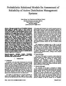
task of making an inference about a new, previously unseen Vote.score. To accomplish this task, we leverage the ground Bayesian Network [Get02] induced by a PRM. Briefly, a Bayesian Network is constructed from a database using the link structure of the associated PRM’s dependency graph, together with the parameters that are associated with that dependency graph. For example, for the PRM in Figure 1(a), if we needed to infer the Score value for a new Vote object, we simply construct a ground Bayesian Network using the appropriate attributes retrieved from the associated Person and Movie objects; see Figure 1(b). The PRM’s class-level parameters for the various attributes are then tied to the ground Bayesian Network’s parameters, and standard Bayesian Network inference procedures can be used on the resulting network [Get02].

3

The following definition summarizes the key elements of a PRM: Definition 1 ([Get02]) A probabilistic relational model (PRM) Π for a relational schema S is defined as follows. For each class X ∈ X and each descriptive attribute A ∈ A(X), we have a set of parents Pa(X.A), and a conditional probability distribution (CPD) that represents PΠ (X.A|P a(X.A))

In this section we describe our approach to extending standard PRMs to include class hierarchies. The concept of learning PRMs with class hierarchies is introduced in [Get02].

3.1 2.1

Applying Standard PRMs to the EachMovie Dataset

PRMs provide an ideal framework for capturing the kinds of dependencies a recommender system needs to exploit. In general, model-based collaborative filtering algorithms try to capture high-level patterns in data that provide some amount of predictive accuracy. For example, in the EachMovie dataset, one may want to capture the pattern that young males tend to rate Action movies quite highly, and subsequently use this dependency to make inferences about unknown votes. PRMs are able to model such patterns as class-level dependencies, which can subsequently be used at an instance level to make predictions on unknown ratings. — i.e., how will George vote on SoM. In order to use a PRM to make predictions about an unknown rating, we must first learn the PRM from data. In our experiments we use the PRM learning produce described in [FGKP99], which provides an algorithm for both learning a legal structure for a PRM and estimating the parameters associated with that PRM. Figure 1(a) shows a sample PRM structure learned from the EachMovie dataset. With the learned PRM in hand, we are left with the

Hierarchical Probabilistic Relational Models

Motivation

The collaborative filtering problem presents two major motivations for hPRMs. First, in the above model, Vote.Score can depend on attributes of related objects, such as Person.Age, but it is not possible to have Vote.Score depend on itself in any way. This is due to the fact that the class-level PRM’s dependency structure must be a directed acyclic graph (DAG) in order to guarantee that the instance-level ground Bayesian Network forms a DAG [FGKP99], and thus a wellformed probability distribution. Without the ability to have Vote.Score depend probabilistically on itself, we lose the ability to have a user’s rating of an item depend on his rating of other items or on other user’s ratings on this movie. For example, we may wish to have the user’s ratings of Comedies influence his rating of Action movies, or his rating of a specific Comedy movie influence his ratings of other Comedy movies. Second, in the above model we are restricted to one dependency graph for Vote.Score; however, depending on the type of object the rating is for, we may wish to have a specialized dependency graph to better model the dependencies. For example, the dependency graph for an Action movie may have Vote.Score depend on Vote.PersonOf.Gender, whereas a Documentary may depend on Vote.PersonOf.Age.

Figure 1: (a) Standard PRM learned on EachMovie dataset (b) Ground Bayesian Network for one Vote object erence slots. For example, if we specialize the M ovie class, we implicitly specialize the related V ote table into a hierarchy as well. For example, in Figure 3, the V ote class is refined into four different pseudo-classes, each associated with one of the hierarchy elements in basic(H[X]). Definition 2 A Hierarchical Probabilistic Relational Model (hPRM) ΠH is defined as: • A class hierarchy H[X] = (C[X], ≺) • A set of basic, leaf-node elements basic(H[X]) ∈ H[X] Figure 2: Sample class hierarchy

3.2

Overview

To address the problem described above, we must introduce a class hierarchy that applies to our dataset, and modify the PRM learning procedure to leverage this class hierarchy in making predictions. In general, the class hierarchy can either be provided as input, or can be learned directly from the data. We refer to the class hierarchy for class X as H[X]. Figure 2 shows a sample class hierarchy for the EachMovie domain. H[X] is a DAG that defines an IS-A hierarchy using the subclass relation ≺ over a finite set of subclasses C[X] [Get02]. For a given c, d ∈ C[X], c ≺ d indicates Xc is a direct subclass of Xd (and Xd is a direct superclass of Xc ). The leaf nodes of H[X] represent the basic subclasses of the hierarchy, denoted basic(H[X]). In this paper we assume all objects are members of a basic subclass, although this is not a fundamental limitation of hPRMs. Each object of class X has a subclass indicator X.Class ∈ basic(H[X]), which can either be defined manually or learned automatically by a supplementary algorithm. By defining a hierarchy for a class X in a PRM, we also implicitly specialize the classes that are reachable from X via one or more ref-

• A subclass indicator attribute X.Class basic(H[X])

∈

• For each subclass c ∈ C[X] and attribute A ∈ A(X) we have a specialized CPD for c denoted P (X c .A|P ac (X.A)) • For every class Y reachable via a reference slot chain from X we have a specialized CPD for c denoted P (Y c .A|P ac (Y.A)) The algorithm for learning an hPRM is very similar to the algorithm for learning a standard PRM. Instead of dealing with the standard set of classes X when evaluating structure quality and estimating parameters, our hPRM algorithm dynamically partitions the dataset into the subclasses defined by H[X]. For inference, a similar technique is used, as for any given instance i of a class, i’s place in the hierarchy is flagged through X.Class; using this flag it is possible to associate the proper CPD with a given class instance. 3.3

Applying hPRMs to the EachMovie Dataset

Applying the hPRM framework to the EachMovie dataset requires a hierarchy to be defined, which is

Figure 3: Example hPrm for EachMovie dataset then used to build an hPRM that is ultimately used to make predictions for unknown votes.

ing task for the EachMovie dataset. We also compare our results to other CF algorithms.

In our experiments we automatically learn a hierarchy to be used in the learning procedure. In the EachMovie database, a movie can belong to zero or more of the following genre categories: action, animation, art foreign, classic, comedy, drama, family, horror, romance, thriller.

4.1

We denote the set of genres that a movie belongs to with G. For example, G(WhenHarryMetSally) = {comedy, drama, romance}. To build our hierarchy dynamically, we first enumerate all combinations of genres that appear in the EachMovie database, and denote this set G. We then proceed to greedily partition G by the number of movies a given element of G is associated with until we reach a predefined limit of k partitions. We define one additional noisy-or –type partition that is used to for movies that do not fall into one of the predefined partitions. This partition, together with the other k partitions, are used to create a k + 1-element hierarchy. With the hierarchy defined, the hPRM is applied to the EachMovie dataset just as the standard PRM model was in Section 2.1, with the exception that the learning procedure is modified as outlined above.

4

Experimental Results

In this section we outline our results in applying both standard PRMs and hPRMs to the collaborative filter-

Experimental Design

One of the main challenges in designing an experiment to test the predictive accuracy of a PRM model is in avoiding resubstitution error. If a PRM is learned on the entire EachMovie database, and subsequently used to make predictions on objects from the same database, we are using the same data for testing as we used for training. We address this issue by applying a modified crossvalidation procedure to the dataset. While the traditional method of dividing data into cross-validation folds cannot be applied directly to a relational database, we extend the basic idea to a relational setting as follows. For n-fold cross validation, we first create n new datasets D1 . . . Dn with the EachMovie data schema. We then iterate over all the objects in the P erson table, and randomly allocate the individual to one of Di ∈ Di . . . Dn . Finally, we add all the V ote objects linked to that individual, and all the M ovie objects linked to those V ote objects, to Di . When this procedure is complete, n datasets with roughly balanced properties (in terms of number of individuals, number of votes per person, etc.) will have been created. In our experiments we use 5-fold cross validation.

4.2

Evaluation Criteria

In this paper we adopt the Absolute Deviation metric [MRK97, BHK98] to assess the quality of our CF algorithms. We divide the data into a training and test set using the method described above, and build a PRM using the training data. We then iterate over each user in the test set, allowing each user to become the active user. For the active user we then iterate over his set of votes, Pa , allowing each vote to become the active vote; the remaining votes are used in the PRM model (if needed). The predicted vote for the active user a on movie j is denoted pa,j , whereas the actual vote is denoted va,j . The average absolute deviation, where ma is the number of vote predictions made, is: Sa =

1 ma

X

|pa,j − va,j |

Standard PRMs Algorithm CR BC BN VSIM PRM

Absolute Deviation 1.257 1.127 1.143 2.113 1.26

Table 1: Absolute Deviation scoring results for EachMovie dataset. Lower scores are better. In our experiments we were able to achieve an absolute deviation error of 1.26. For comparison, we have included the results from [BHK98]; in this paper four CF algorithms were tested: correlation (CR), Bayesian Clustering (BC), a Bayesian Network model (BN), and Vector Similarity (VSIM). We have elected to include the results from [BHK98] where algorithms were given two votes out of the non-active votes to use in making the prediction, since the standard PRM model does not have any direct dependency on other V otes. In this experiment standard PRMs are able to outperform the VSIM algorithm, and is competitive with the correlation-based algorithm. However, both Bayesian Clustering and the Bayesian Network model have superior results in this context. 4.4

Algorithm CR BC BN VSIM hPRM

Absolute Deviation 0.994 1.103 1.066 2.136 1.060

Table 2: Absolute Deviation scoring results for EachMovie dataset. Lower scores are better.

(1)

j∈Pa

The absolute deviation for the dataset as a whole is arrived at by averaging this score over all the users in the test set of users. 4.3

dataset. In our experiment we set the size of the hierarchy to be 12. Our greedy partitioning algorithm arrived at the following basic classes: drama, comedy, classic, action, art-foreignDrama, thriller, romancecomedy, none, family, horror, actionThriller, other.

Hierarchical PRMs

The first part of the experiment for hPRMs was constructing a class hierarchy from the EachMovie

By applying hPRMs to the EachMovie dataset, we are able to reduce the absolute deviation error from 1.26 (with standard PRMs) to 1.06. Again, for comparison we include results from [BHK98]; however, in since hPRMs are able to leverage other votes the user has made in making predictions, we use the All-But-One results presented in [BHK98], where the prediction algorithm is able to use all of the active user’s votes (except for the current active vote) in making a prediction. As one can see by comparing Table 1 to Table 2, including the additional voting information results in a substantial reduction in error rate for most of the other four algorithms. hPRMs not only provide a significant performance advantage over standard PRMs, but are also able to outperform all but one of the other four algorithms.

5

Future Work

In this paper we learned a fairly broad hierarchy based on various sub-genres in the EachMovie dataset. However, hPRMs allow for arbitrarily specific class hierarchies, where a leaf-node entry for H[X] might be a handful (or even just one) movie. This could be exploited when there are certain indicator movies in a Genre that may accurately predict a user’s votes on other movies in that (or other) Genres, and that furthermore most users have seen. For example, whether a user likes science fiction movies or not, they have likely seen the Star Wars Trilogy; this fact could be leverage by making the Star Wars movies a basic subclass in the class hierarchy, and subsequently used to learn new dependencies of the type if a user likes the Star Wars movies, they will in general like science fiction movies. Learning such a hierarchy is a challenging task that would likely significantly improve the performance of hPRMs.

6

Conclusion

In this paper we outlined a framework for modelling the collaborative filtering problem with PRMs. We model the CF problem first using a standard PRM, then we extend model to account for hierarchical relationships that are present in the data. hPRMs improve the expressiveness and context-sensitivity of standard PRMs, and also realize real-world performance benefits. Acknowledgements

[MRK97] Bradley N. Miller, John T. Riedl, and Joseph A. Konstan. Experience with GroupLens: Making Usenet useful again. In USENIX, editor, 1997 Annual Technical Conference, January 6–10, 1997. Anaheim, CA, USA, pages 219–233, Berkeley, CA, USA, 1997. USENIX. [UF98a]

L. Ungar and D. Foster. Clustering methods for collaborative filtering, 1998.

[UF98b]

L. Ungar and D. Foster. A formal statistical approach to collaborative filtering, 1998.

Both authors thank Lise Getoor for useful discussions and encouragement (as well as access to her software), Dale Schuurmans for his advice on this project, and thank NSERC and the Alberta Ingenuity Centre for Machine Learning for funding. Some of this work was done when RG was on sabbatical visiting CALD/CMU.

References [Aha97]

D. Aha. Special issue on “Lazy Learning”. Artificial Intelligence Review, 11(1– 5), February 1997.

[BHK98]

John S. Breese, David Heckerman, and Carl Kadie. Empirical analysis of predictive algorithms for collaborative filtering. In UAI98, pages 43–52, 1998.

[CHM97] David Maxwell Chickering, David Heckerman, and Christopher Meek. A Bayesian approach to learning Bayesian networks with local structure. In UAI97, pages 80– 89, 1997. [Eac]

http://research.compaq.com/SRC/eachmovie/.

[FGKP99] Nir Friedman, Lise Getoor, Daphne Koller, and Avi Pfeffer. Learning probabilistic relational models. In IJCAI, pages 1300– 1309, 1999. [Get02]

L. Getoor. Learning Statistical Models from Relational Data. PhD thesis, Stanford University, 2002.

[KP98]

D. Koller and A. Pfeffer. Probabilistic frame-based systems. In Proc. of the Fifteenth National Conference on Artificial Intelligence, pages 580–587, Madison, WI, 1198.

[Mit97]

Tom M. Mitchell. McGraw-Hill, 1997.

Machine Learning.