IEEE TRANSACTIONS ON POWER SYSTEMS, VOL. 29, NO. 5, SEPTEMBER 2014
2229
Hierarchical Spectral Clustering of Power Grids Rubén J. Sánchez-García, Max Fennelly, Seán Norris, Student Member, IEEE, Nick Wright, Graham Niblo, Jacek Brodzki, and Janusz W. Bialek, Fellow, IEEE
Abstract—A power transmission system can be represented by a network with nodes and links representing buses and electrical transmission lines, respectively. Each line can be given a weight, representing some electrical property of the line, such as line admittance or average power flow at a given time. We use a hierarchical spectral clustering methodology to reveal the internal connectivity structure of such a network. Spectral clustering uses the eigenvalues and eigenvectors of a matrix associated to the network, it is computationally very efficient, and it works for any choice of weights. When using line admittances, it reveals the static internal connectivity structure of the underlying network, while using power flows highlights islands with minimal power flow disruption, and thus it naturally relates to controlled islanding. Our methodology goes beyond the standard -means algorithm by instead representing the complete network substructure as a dendrogram. We provide a thorough theoretical justification of the use of spectral clustering in power systems, and we include the results of our methodology for several test systems of small, medium and large size, including a model of the Great Britain transmission network. Index Terms—Clustering, power system analysis computing.
I. INTRODUCTION
T
HE idea of decomposing (partitioning, tearing, splitting, clustering) a power network into smaller parts goes back to the concept of diakoptics introduced by G. Kron in the 1950s [1], and it was followed by many others, e.g., [2]–[4]. The initial motivation was the limited memory and computation speed of early computers. Later on, the advent of parallel computing resulted in a very significant research effort aimed at splitting the power system model into smaller parts to be solved in parallel. Decomposing large interconnected networks into looselyconnected zones that could be more easily managed often uses the concept of electrical cohesiveness as expressed by electrical distance between network nodes [5] to define network zones. Generally, network splitting can enable a flexible, distributed and adaptable power system control that utilizes the concept of smart grids [6].
Manuscript received June 21, 2013; revised November 29, 2013; accepted February 09, 2014. Date of publication March 17, 2014; date of current version August 15, 2014. This work was supported by the EPSRC grants EP/G059101/1 and EP/G060169/1. Paper no. TPWRS-00806-2013. R. J. Sánchez-García, M. Fennelly, N. Wright, G. Niblo, and J. Brodzki are with the School of Mathematics, University of Southampton, Southampton SO17 1BJ, U.K. (e-mail:
[email protected]). S. Norris and J. W. Bialek are with the School of Engineering and Computing Sciences, Durham University, Durham DH1 2PE, U.K. (e-mail: Janusz.
[email protected]). Color versions of one or more of the figures in this paper are available online at http://ieeexplore.ieee.org. Digital Object Identifier 10.1109/TPWRS.2014.2306756
Network splitting is also used in controlled islanding that aims to prevent the spreading of large-area blackouts. The most popular methodologies proposed include keeping together slow-coherent generators to avoid the loss of transient stability [7] and graph-search based approaches, e.g., [8], [9]. Recently a novel methodology of spectral clustering has been proposed for controlled islanding that is based on recent advances in graph theory [10], [11]. The main contribution of this paper is to adapt the spectral clustering methodology [12], [13] to the context of power transmission networks, and explain how this technique can be used to provide a real-time, versatile, analytical or visualization tool for power transmission systems. Our methodology reveals the internal structure of a given network with respect to any choice of electrical parameter that can be associated to a transmission line, such as line admittance, power flow or other. It may also take a preferred number of clusters as input, or this number can be obtained directly from the data. The output is a hierarchical clustering of the network according to the connection strengths given by the chosen weighting. This may be thought of as a functional decomposition of the system into smaller subsystems of highly connected buses. Our methodology goes beyond bisection or recursive bisection techniques by providing an all-in-one decomposition of the network into any number of clusters. Indeed, we keep all the underlying hierarchical substructure, instead of just a partition of the network, by using a hierarchical clustering algorithm as our final step. This way we are able to represent simultaneously the different levels in the clustering, and reveal the scale-dependence of the resulting data, which represents the functional hierarchy of the network. This paper should be thought as a proof-of-concept of the underlying spectral clustering technique in the power engineering context, and we have taken special care in explaining its mathematical basis. We illustrate the potential of our methodology in a small test network in full detail, and in other larger test networks in some detail. The paper is the result of a collaboration between power engineers and mathematicians, as we strongly believe that there is a wealth of knowledge in graph and operator theory that is not widely known in the power engineering community and which could be usefully employed to solve practical power engineering problems. This paper is an attempt in that direction. II. PRELIMINARIES A. Graphs Representing a Power Transmission Grid 1) Terminology and Notation: A power network can be naturally represented as a graph: vertices (nodes) represent buses, and edges (links) represent electrical connections. We
0885-8950 © 2014 IEEE. Translations and content mining are permitted for academic research only. Personal use is also permitted, but republication/ redistribution requires IEEE permission. See http://www.ieee.org/publications_standards/publications/rights/index.html for more information.
2230
IEEE TRANSACTIONS ON POWER SYSTEMS, VOL. 29, NO. 5, SEPTEMBER 2014
write for a graph with vertex set and edge set . In what follows we will only consider simple graphs, where no loops and no multiple edges are allowed. This assumption does not restrict the generality of our consideration as multiple edges can be replaced by equivalent single edges. Since the graph is finite and simple, we can write , where is the number of vertices (nodes), and , where represents an edge (a transmission line or a transformer) from vertex to vertex . Since spectral clustering ignores edge directions, we will assume that all graphs are undirected: if and only if . 2) Edge Weights: The topological structure of the graph does not capture the functional information about the power grid. To include this information, we use edge weights. An edge weight is a function such that 1) for all ; 2) if ; 3) . We use the notation if , and for the so-called weighted vertex degree. The purely topological structure of the graph is returned when we select the weight function for all , recovering the classical adjacency matrix in this case. Note that the edge weights must be nonnegative and symmetric to have a Laplacian (see Section II-B). 3) Weights in Power Grids: To study the functional structure, in a very restricted sense, of a power grid we may use the following edge weight functions: • Topology: for all ; this measures pure connectivity of the network. • Admittance: , where and are the line resistance and reactance respectively; this measures the strength of connections (electrical distance). In this paper we will use the DC network model in which these weights are . • Average power flow: , where is the (real) power flow from to (if the network is lossless this is simply the power flow ); this weight measures the importance of a line in a given operating condition—a small flow means that the line is more likely to be removed when clustering. Note that the first two weights are static, i.e., they are constant for a given power system, while the power flow is dynamic, as it changes according to actual operating conditions. Edge weights can be interpreted as a penalty for cutting the corresponding line when clustering, but also as a measure of the connection strength, as strongly connected vertices are more likely to be clustered together. Thus the admittance based clustering will reveal the internal structure (electrical distance) of the network while the power flow based clustering will reveal islands which, when separated, disrupt as least as possible the power flow in the network, and thus can be especially useful for preventive islanding purposes [11].
kinds of Laplacian matrix that can be associated with an undirected weighted simple graph . 1) Unnormalized Laplacian: The Laplacian of is the matrix defined as
B. Graph Laplacians The Laplacian matrix is widely used in graph theory and it has a clear power engineering interpretation. There are two main
if ; if and otherwise.
;
(1)
It is a real symmetric matrix with non-positive entries outside the diagonal, and the sum of each column (or row) is zero. If the weights are equal to inverse line reactances (using the DC network model), then the unnormalized Laplacian is simply equal to the well-known nodal admittance matrix (neglecting shunt susceptances). There is no established power engineering interpretation of the Laplacian when the weights are equal to power flows. 2) Normalized Laplacian: The normalized Laplacian is the matrix , where is the diagonal matrix with nonzero entries . That is, if if
; and
;
(2)
otherwise. The normalized Laplacian is scale-independent, and it is more advantageous for clustering purposes (see Section IV-A). C. Eigenvalues of the Laplacian The eigenvalues of the (normalized or unnormalized) Laplacian matrix satisfy the following key properties [14]: 1) all the eigenvalues are nonnegative real numbers; 2) 0 is an eigenvalue with multiplicity equal to the number of connected components (islands) in the graph. We write the eigenvalues of as , and the eigenvalues of as . From property (2) above, we know that , or , if and only if is connected. From now on we will assume that our graph is connected. The eigenvalues of are scale-dependent and have no a priori upper bound (multiplying all weights by a scalar multiplies all the eigenvalues by the same scalar). However, the eigenvalues of satisfy the inequality for all . III. SPECTRAL CLUSTERING A. Introduction and Terminology By clustering we mean the identification of groups of vertices in a graph (called clusters) such that the vertices in a cluster are highly connected among themselves (taking edge weights into consideration) but weakly connected to vertices in other clusters. By spectral clustering we mean any clustering procedure that uses the Laplacian eigenvalues and eigenvectors [12]. A theoretical justification for spectral clustering is deferred to Section III-C below. The general idea is to use the first eigenvectors of a Laplacian to give geometric coordinates to the vertices in , for some . Namely, these coordinates are the rows of the matrix whose columns are the eigenvectors of the
SÁNCHEZ-GARCÍA et al.: HIERARCHICAL SPECTRAL CLUSTERING OF POWER GRIDS
2231
smallest eigenvalues. The resulting data points are then clustered using some standard clustering algorithm developed for point clouds in Euclidean space (normally -means). Spectral clutering will try to create balanced clusters of approximately equal volume, as explained later. To measure the quality of a partition, we need to introduce a quantity called subgraph expansion. B. Subgraph Expansion A subgraph is the graph induced by a subset of vertices : the vertices are , and the edges are such that . In agreement with the accepted power engineering terminology, an island will be a subgraph of spanned by a subset of the vertex set . (Note that a priori islands do not need to be connected.) We implicitly consider only non-trivial islands ( and ). The volume of an island spanned by a subset is by definition the sum of the degrees of its vertices: (3) Note that the volume of is determined by the weights associated with the vertices in , and not just their number. The boundary of is the sum of the weights of the edges between vertices in and vertices not in (i.e., the sum of weights of the tie-lines linking with the rest of the network):
Fig. 1. Power flow in the IEEE 39-bus test case, and clustering into four islands with our methodology (see Section V-A). The islands are colored and named Green, Red, Yellow and Blue. See Table II for the boundaries, volumes and expansion ratios of these islands. Note that, although shown in the figure, spectral clustering ignores the power flow directions. Observe that the island but maximal expanwith just bus 12 has the smallest boundary , as its boundary amounts to all its volume. sion
The best -partition overall (with respect to expansion) is the minimum over all possible -partitions of the graph: (7)
(4) To measure the quality of an island we will use the ratio of the size of the boundary to the volume of . For this we define the expansion of as the quotient (5) The smaller the expansion of , the better the island is considered to be in terms of clustering: a “good” island will contain vertices highly interconnected among themselves (large ), and weakly connected with the rest of the network (small ). See Fig. 1 and Table II for examples of the concepts of boundary, volume and expansion. Note that minimizing the boundary alone, instead of a ratio, gives inadequate solutions, as the island with smallest boundary in a network consists just of the vertex with smallest degree (see Fig. 1, caption). Hence minimizing the boundary without additional constraints gives rise to spurious solutions.
This quantity is called the -way expansion constant of the graph . A brute-force approach to finding an optimal partition (attaining the minimum above) is not computationally feasible for large networks, and indeed search problems on graphs like this one are generally NP-hard [15]. Spectral clustering provides instead an approximate solution, with a computational complexity depending only on the computation of the first eigenvalues and eigenvectors of a Laplacian matrix (at most cubic on for a real, symmetric matrix of size ). The Cheeger inequality measures how close this approximate solution is to the optimal solution, and how good overall this optimal solution is, that is, how well the graph admits a -partition. For , the Cheeger inequality is [14] (8) and this classical inequality has been recently generalized to , in the following asymptotic sense [13]: arbitrary (9)
C. Cheeger Inequality The Cheeger inequality is one of the main theoretical justifications of the spectral clustering methodology [12]. Since we measure the quality of an island by its expansion , we will measure the quality of a -partition (i.e., a partition into clusters) by the maximum expansion among the islands: (6)
In fact, the right-hand sides of (8) and (9) are obtained by using spectral clustering with respect to the normalized Laplacian. On the left-hand side, the value represents the minimal value of the expansion of any -partition of the network. Therefore, the smaller is, the closer the approximate spectral clustering solution is to the optimal one, and the better this optimal solution is overall. If is large, the graph will not admit a good -partition.
2232
IEEE TRANSACTIONS ON POWER SYSTEMS, VOL. 29, NO. 5, SEPTEMBER 2014
An important observation is that clustering a network into several clusters while minimizing the overall expansion (6) is equivalent to trying to balance the volume of all the clusters. IV. SPECTRAL CLUSTERING METHODOLOGY A. Rationale The essence of the spectral clustering methodology is to use the first eigenvectors of a graph Laplacian to give coordinates to the vertices in -dimensional Euclidean space . This so-called spectral -embedding should reveal a clustering into islands. There are a number of variants of this general methodology. A first choice is whether to use the normalized or the unnormalized Laplacian [12]. There are a number of reasons why it is generally more advantageous to use the normalized Laplacian , particularly for arbitrarily weighted networks [13], [16], and indeed we found in all our simulations that eigenvectors of the normalized Laplacian performed better in terms of clustering solutions. This justifies Steps 1 and 2 in our algorithm (see Section IV-B below). It is known that when using the eigenvalues of , there is an extra normalization step after the spectral embedding, in which the vectors must be normalized to have all length 1 [12], [13]. This justifies Step 3 in Section IV-B. A second choice is that of a clustering algorithm for point clouds in Euclidean space, in order to identify the clusters revealed by the spectral -embedding when , where visualization is difficult. The standard choice is the -means algorithm [12]. However, this procedure has a few deficiencies from the point of view of the overall control of the clustering process. First, one needs to decide beforehand how many clusters one wishes to obtain, normally using the spectral embedding in to obtain clusters. Secondly, this method does not allow one to encode the complete clustering structure of the original network but rather output a single partition of the network. Thirdly, the clustering algorithm in Euclidean space ignores the fact that the points represent vertices in a graph, that is, it ignores the edge information. To overcome these shortcomings, we use hierarchical clustering instead of the more standard -means algorithm [17]. This reveals a fine structure of the grid at various levels of resolution simultaneously, which we encode using a dendrogram. A dendrogram is a tree diagram (such as Fig. 5) that encodes the hierarchical structure in the spectral embedding. The bottom “leaves” represent the individual vertices (buses), considered as initial clusters of size 1. At each step up the tree, the closest clusters are merged together, measuring the distance between clusters as the shortest pairwise distance between points in different clusters. A dendrogram represents the hierarchical structure of the network at all levels at once, and indeed a specific -partition, for some , can be recovered by “cutting” the dendrogram at level from the root (see Fig. 5 for an example). To deal with the third shortcoming, we equip the graph with a metric induced by the spectral embedding that takes into account the edge information. Assume that is the normalized coordinate associated to the th vertex [see (11)]. Then we set the edge distance if vertices and
Fig. 2. Eigengaps (left) and relative eigengaps (right) for the power flow based Laplacian in the IEEE 39-bus test case.
are connected in the graph, and, in general, is the minimum distance over paths connecting to in the graph, where the distance over a path is the sum of the edge distances. The main advantage is that it only allows merging of islands already connected by at least one edge. We call this the metric induced on the graph by the embedding. One final refinement is that we compute the distances over the sphere instead of the straight-line distance, since we are clustering a point cloud on the -dimensional sphere. The last few paragraphs explain and justify Step 4 in our algorithm. In this way, we obtain a clustering with a fascinating scale-dependence which will allow us to “zoom into” clusters to reveal their finer structure. This new level of control will exhibit the true functional structure of the grid as a whole at various levels of resolution. In particular, the output of our algorithm is not just a partition of the network (although such partitions can be readily obtained) but rather the spectral embedding hierarchical clustering structure, encoded and visualized using a dendrogram. There is still a choice of dimension in which to embed the network, which is turn relates to the preferred number of clusters we seek to find. This number may be problem dependent, for instance the preferred volume of the clusters, but otherwise we would like to know the optimal dimension for the spectral embedding. A common criterion is to use the eigengaps, that is, the difference between two consecutive eigenvalues (recall that a good -partition exists if is small). Since we are interested in the smallest eigenvalues, we use an eigenvalue difference relative to their size: (10) A high value of (see Fig. 2 for an example) indicates that the network admits a good decomposition into at least islands, and that this will be revealed by the spectral embedding in dimension . Note that the hierarchical clustering will nevertheless keep track of the subcluster structure within each cluster, beyond simply a -partition. Therefore, in absence of any other criterion, we will use a high value of to choose the dimension for the spectral embedding (Step 0). B. Algorithm Let vertices.
be an undirected weighted graph with
SÁNCHEZ-GARCÍA et al.: HIERARCHICAL SPECTRAL CLUSTERING OF POWER GRIDS
TABLE I TOPOLOGY, EIGENBASIS COMPUTATION TIMES
Step 0 (Spectral Dimension) Choose with a high value of , the relative eigengap in (10). Step 1 (Normalized Laplacian) If is the matrix of edge weights, define where , , and . Step 2 (Spectral embedding) Use the first eigenvectors of the normalized Laplacian to give coordinates to the vertices of the graph in . (If is the matrix whose columns are the first eigenvectors, then the is the th row of .) Step 3 (Normalization) Normalize the vectors to have length 1 in : (11)
2233
smaller electrical distance. The main difference is that the spectral distance organizes the vertices such that clusters are revealed, hence it is a global distance with respect to an additional clustering parameter . Mathematically, Thevenin’s impedance takes into account all eigenvectors of the unnormalized Laplacian (computing all eigenvalues and eigenvectors of a diagonalizable matrix is equivalent to computing its inverse), while the spectral embedding uses only the smallest eigenvalues. Note also that the spectral distance is associated to a spectral embedding into Euclidean space, which provides an additional geometric or spatial insight, while Thevenin’s impedance is a purely numerical measure with no additional spatial information. V. TEST CASE: IEEE 39-BUS TEST SYSTEM We illustrate our methodology on the IEEE 39-bus test system in full detail. In the next section we will apply the methodology to other systems and summarize the main findings. We start with the spectral clustering based on the power flow Laplacian and later compare the results to the admittance based Laplacian. All the numerical results were performed on Matlab R2011b (64bit) on an iMac 3.06-GHz processor with 4 Gb of RAM. A. Power Flow Laplacian
(This amounts to a radial projection onto the -sphere .) Step 4 (Hierarchical clustering) Compute the dendrogram of the points with respect to the metric induced on the graph by the embedding, as explained in Section IV-A. C. Algorithmic Complexity The largest computational time occurs in Step 2, the computation of the eigenbasis of a matrix of size , which is at most cubic in . We used Matlab (see Section V below), which in turn employs a Cholesky factorization algorithm, to compute the eigendecomposition of a positive-definite symmetric matrix. In practice, this computation took at most a fraction of a second in all our test cases, mostly due to the sparsity of the matrices involved (see Table I for mean times over 100 trials, and Section V for software and hardware details). D. Physical Interpretation of the Spectral Distance The spectral -embedding provides a distance function between buses and it is interesting to compare it with the Thévenin’s equivalent impedance, which is a standard measure of electrical distance. The latter can be calculated by inverting the admittance matrix (i.e., the Laplacian with weights equal to admittances) which suggests a connection with the spectral distance when admittances are used as weights. In general, the distance obtained by inverting the Laplacian is often correlated to the unnormalized spectral embedding, but there is no known direct mathematical relation [12]. In practice, we found high linear correlation factors between the electrical and the spectral distance for the unnormalized admittance based Laplacian: 0.89, 0.82 and 0.87 for the IEEE 39, IEEE 118 and GB test cases, respectively, for suitable choices of . This is to be expected, as high connectivity between buses results in
We performed the spectral clustering analysis of the IEEE 39-bus test system based on the DC power flows shown in Fig. 1. We first concentrate on dimensions 2 and 3, where we can visualise the embeddings. More generally, we would use the relative eigengaps (10) to determine the optimal spectral dimension , and, if , as visualization is harder, a dendrogram to represent the hierarchical internal structure. Step 0 (Spectral dimension) We choose a spectral dimension from the peaks in the relative eigengaps (Fig. 2). In this case the peaks at ,5 suggests using dimensions 3 or 5 to reveal the underlying clustering structure. We would choose , although we will do the analyisis for both equals 2 and 3, for illustrative purposes. Steps 1, 2 (Normalized Laplacian, Spectral embedding) We construct the normalized Laplacian with respect to the power flows, compute an orthonormal basis of eigenvectors, and use the first eigenvectors to provide coordinates to the buses in , for and 3. This effectively provides a representation or visualization of the network in (Fig. 3, left), respectively (Fig. 4, left). We can already see a “radial” clustering emerging, that is, points clustering along half-lines emerging from the origin. Step 3 (Normalization) We normalize the coordinates so all the vectors have norm 1, that is, we project onto the unit circle or the unit sphere . This procedure projects the points along radial lines from the origin, revealing the radial clustering structure mentioned above. In Fig. 3, we show the spectral 2-embedding before (left) and after normalizing (right). By visual inspection, we can already see a hierarchical clustering structure emerging, with four clusters and several levels of subclusters of data points (Fig. 3, right). For we obtain points in the 2-dimensional sphere (not shown), although we performed a stereographic projection onto the plane for better visualization
2234
IEEE TRANSACTIONS ON POWER SYSTEMS, VOL. 29, NO. 5, SEPTEMBER 2014
Fig. 5. Dendrogram of the spectral 3-embedding for the IEEE 39-bus test system weighted by power flows. The Blue, Green, Yellow and Red islands (from left to right on the horizontal axis) are recovered at height 1, while cutting at height 3 suggests merging the Green and Red islands for a good 3-partition (cf. Fig. 1 and Table II). Long vertical lines in a dendrogram reveal a good clustering at that level. Fig. 3. Spectral 2-embeddings for the IEEE 39-bus test case and power flows. The right-hand side plot shows the normalized embedding (points lie on a unit circle), with points labelled by bus number, and four discernible clusters are highlighted (Blue, Green, Red and Yellow from top to bottom).
TABLE II PARTITION INTO FOUR (THREE) ISLANDS
B. Revealing the Internal Connectivity of the Network
Fig. 4. Spectral 3-embedding for the IEEE 39-bus test case weighted with power flows (left) and stereographic projection (right). We can visually identify four clusters (colored yellow, blue, green and red clockwise from the top left corner), which are the same as in the spectral 2-embedding (Fig. 3, right). Labels indicate bus number. The right-hand side plot is obtained by normalizing the vectors to length 1, and performing a stereographic projection from the point (1,0,0).
(Fig. 4, right). It is apparent that an even more detailed subclustering structure emerges (see Section V-B). Note that the normalized eigenvectors give points on a semi-circle (Fig. 3, right), respectively, on a semi-sphere (not shown), due to the first eigenvector being , hence the first coordinate of all points always have the same sign. Step 4 (Hierarchical clustering) The chosen dimensions are small enough to allow clustering by simple visual inspection (Figs. 3, 4, right), although the corresponding dendrogram reveals the same clustering information (see Fig. 5). Going back to the original network, we check that these four islands make sense (Fig. 1), and indeed they are connected and have small boundaries relative to their volumes (Table II). It is interesting to compare the expansion ratios found with the theoretical lower bounds for ,4 (see Section III-C): 0.0065 and 0.0226, respectively. That is, the optimal -partition (which cannot be found in general in polynomial time) has an expansion of at least 0.65% resp. 2.26% for ,4, in contrast to the ones we found (in a few miliseconds) of 2.05% and 5.03%, respectively, avoiding an exponential search.
We can exploit the spectral embedding further: by inspection it shows indeed a rich subclustering structure, see Figs. 3 and 4 (right). For example, the relative position of individual buses reflects whether they belong to the “core” of an island or to the “periphery”, in some sense (see bus 9 in Figs. 4-1 for an example). Also, exploring the dendrogram (Fig. 5) we can see that merging the Green and Red islands gives a good 3-partition (cf. Fig. 1 and Table II). Uncovering this further subclustering structure is the main motivation behind the choice of hierarchical clustering in our methodology. The complete hierarchical structure of the network will be encoded in a dendrogram. Although a dendrogram captures the different scales in the data, different choices of the spectral embedding dimension will reveal slightly different partitions, as different spectral embedding dimensions will favor configurations depending on the expected balanced -partition ( clusters of size approximately ). C. Admittance Laplacian We do the same analysis for the admittance based Laplacian. The input is the same network with different weights, now the line admittances shown in Fig. 6. Due to lack of space we show only a network partition using the spectral 3-embedding. The three islands obtained are similar to the ones in Fig. 1 for the power flow Laplacian, as line admittances and power flows are obviously correlated (0.66 linear correlation factor), and indeed constrained by the network topology (the admittance and the power flow between two buses is zero if they are not physically connected). On the other hand, the expansion ratios are higher than the power flow based ones (9.34%, Red; 8.00%, Yellow; 3.28%, Blue), as the power flow weights are more sparse (standard deviation of 212.5 as opposed to 68.6 for the admittance weights). This can be also seen on the Laplacian eigenvalues
SÁNCHEZ-GARCÍA et al.: HIERARCHICAL SPECTRAL CLUSTERING OF POWER GRIDS
Fig. 6. Line admittances in the IEEE 39-bus test system, and three clusters (colored and named Red, Yellow and Blue) identified by our methodology (see main text).
2235
Fig. 8. Alternative power flow in the IEEE 39-bus test system and clustering into four islands (colored and named Red, Green, Yellow and Blue) found with our methodology (see main text). The power flow directions are shown for convenience.
TABLE III RESULTS FOR LARGER SYSTEMS
Fig. 7. Eigenvalues for the power flow based (PL) and admittance based (AL) normalized Laplacians of the IEEE 39-bus test systems (left), and IEEE 118-bus test system (right). The characteristic S-shape comes from the properties of the , , and the multiplicity of eigenvalues: (high multiplicity eigenvalues often come from the underlying network symmetry [18]). The more pronounced this S-shape is, the better -partitions for small are expected in the network. Hence the plots predict better power flow based partitions than admittance based ones in the 39-bus test system, and the opposite in the 118-bus test system.
expansion ratios are 5.20% (Yellow), 3.77% (Red), 3.73% (Green) and 1.11% (Blue). A more detailed analysis of the dendrogram allows to explore the subcluster structure; for example the largest (Blue) island can be further subdivided into two: 1–3, 9, 18, 30, 39 and 4–8, 10–14, 31–32. VI. OTHER TEST SYSTEMS
(Fig. 7, left). Indeed, the theoretical lower bound is higher for the admittance based Laplacian: 1.34%, 1.68% and 2.50% for , 3, 4. D. Alternative Power Flow Laplacian The power flow weighting is dynamic in the sense that it varies depending on the network operation conditions. As the power flows change, so does the spectral embedding, and the corresponding hierarchical structure. As an illustration, we change the generator outputs in the IEEE 39-bus test system to create a different pattern of flows (Fig. 8). In this case, dimension 5 reveals a good clustering structure into at least four islands. The hierarchical clustering information is represented in a dendrogram (not shown), and the specific 4-partition associated to it is given in Fig. 8. All the islands are connected, and they have small boundaries compared to their sizes: the
We have applied our methodology to a larger IEEE test system (118 buses), and one large-scale power transmission network of Great Britain (GB); see Table I for their basic topology. For the IEEE 118-bus test system, we use spectral dimension 8 to produce a hierarchical picture of the network connectivity. As an illustration, we compute the associated partition into 6 islands for both the admittance based and the power flow based analysis (not shown due to lack of space), and we list on Table III the maximal expansion among the islands, as a measure of the partition quality. The better partition for the admittance based weighting cannot be explained by the dispersion of the weights (very similar variation) but it can be seen on the eigenvalue plot (Fig. 7, right). For the GB system, we use dimensions 16 and 32 for the power flows, respectively the line admittances. We compute two examples in each case of partitions obtained at these dimensions
2236
IEEE TRANSACTIONS ON POWER SYSTEMS, VOL. 29, NO. 5, SEPTEMBER 2014
TABLE IV COMPARISON EA AND SC ALGORITHMS
(not shown), and we list their maximal expansion on Table III. The admittance based partitions are much better (in terms of expansion ratios) than the power flow based ones, probably due to the exceptionally large variation in weights (standard deviation of 7117 for line admittances, versus 321 for power flows). We also show on Table III the total computing time, which includes: the computation of the Laplacian, its eigenvectors, the spectral embedding, the normalization, the induced distances, and the dendrogram (Steps 1 to 4 of our methodology). We stress that the computer code we use has not been fully optimised, leaving substantial space for improvement, as we only wanted to demonstrate that our methodology should be considered “realtime”. VII. COMPARISON WITH OTHER METHODOLOGIES Recent work on clustering in the context of power grids [7], [10], [19]–[24] aims at providing a partition solution and it is often application-specific. In contrast, our methodology reveals the hierarchical connectivity structure beyond clustering (in particular, it provides a distance function; see Section IV-D) without any further constraints. Therefore, our technique is closest in philosophy to that of [5], although note that we can use any electrical parameter beyond electrical distances, including dynamic criteria such as power flows. Here we carry out an explicit comparison of our method (used as a partitioning tool) to that of [25], since that article builds on [5], and it provides a testable partitioning algorithm. We consider the two test cases treated in [25]: the IEEE 118-bus test system and 3 clusters, and a Polish network of 2383 buses (1733 buses after removing leaf-nodes) and 5 clusters. We carried out our spectral algorithm (SC) with weights equal to line admittances, and compared the solutions to those of the evolutionary algorithm (EA) in [25], with respect to both quality measures: the fitness score in [25], and our measure of expansion, (5), which represents the connectivity of an island relative to its volume. The results are explained below, and summarized on Table IV. For the 118-bus test system, our solution in dimension has slightly (1%) worse fitness, and better (smaller) expansion ratios. Indeed, both solutions are identical up to four buses. For the Polish system, our solution in dimension has a slightly (3.6%) worse fitness, and better expansion ratios. The results are not surprising, as the fitness score in [25] resembles what the spectral algorithm tries to achieve: high intra-cluster connectivity, low inter-cluster connectivity, balanced cluster size, and the ideal number of clusters is controlled by the parameter (spectral dimension). The main difference is that the fitness score is defined with respect to electrical distances, and the expansion ratios with respect to the spectral
distances resulting from line admittances. Nevertheless, as pointed out in Section IV-D, these two are highly correlated. It is noteworthy that our spectral algorithm performs well with respect to an extrinsic (although correlated) quality measure while outperforming with respect to expansion ratio, which is precisely the measure it aims to optimise. In terms of computation times, for the Polish network our algorithm needed about 15 s in our desktop computer to calculate all spectral embeddings up to dimension (in a non-optimized code), and then less than 3 s to find a clustering solution in each dimension. For the 118-bus case the complete computation was done in a fraction of a second. On the other hand, the complexity of genetic algorithms typically depends on the size of the initial population, the number of iterations, and the number of crossovers at each iteration [26]. VIII. CONCLUSION We have presented an efficient algorithm that uses spectral and hierarchical clustering to reveal the internal connectivity structure of a network representing a power grid, with respect to any choice of electrical parameter associated to the transmission lines. We have used power flows and line admittances to illustrate our methodology, in three test systems of small, medium and large size. In addition, we have benchmarked our algorithm, used as a partitioning tool, with respect to a competing technique. Using the power flows as weights is more useful in applications that are dynamic, in the sense that they depend on actual operating conditions. One application is preventive islanding [11], as the clustering tries to minimize the disruption of power flows caused by cutting through tie-lines linking the clusters, but a fascinating possibility could be to use it in a control room as a method of visualizing actual operating conditions. Different nodes in the system would come closer together, or disperse, depending on their loading, hence revealing the power flow loading pattern and structure. Hierarchical spectral clustering can also be done using line admittances when the grid connectivity, as expressed by the electrical distance, is of more interest. This clustering therefore reveals a static internal structure of the network. We used dendrograms to organize and visually represent the hierarchical structure of a network, particularly in dimensions greater than 3. This goes beyond the more standard -means algorithm, and our methodology reveals a complete functional hierarchical substructure of the network beyond a simple partition. In particular, the dendrogram retains information about further subdivisions (or amalgamations) into smaller (larger) islands. We believe that the spectral embedding and associated dendrogram are the correct way of representing a network in terms of internal connectivity with respect to a specific set of edge weights. This may serve as a starting point of further analysis, by reducing the search space, and provide a geometric insight on the functional hierarchy of the network. In particular, exploring the dendrogram and the original network we can fine-tune the details depending on the specific application we are considering. We explained the underlying mathematical theory in detail with the aim to convey the enormous potential of the spectral
SÁNCHEZ-GARCÍA et al.: HIERARCHICAL SPECTRAL CLUSTERING OF POWER GRIDS
clustering methodology, when applied carefully, in the power engineering context. ACKNOWLEDGMENT The authors would like to thank E. Cotilla-Sanchez for kindly providing the data used in Section VII, and M. Battarra for discussions on genetic algorithms. REFERENCES [1] G. Kron, Diakoptics: The Piecewise Solution of Large-Scale Systems. New York, NY, USA: MacDonald, 1963, vol. 2. [2] H. H. Happ, Piecewise Methods and Applications to Power Systems. New York, NY, USA: Wiley, 1980. [3] J. H. Chow, Time-Scale Modeling of Dynamic Networks With Applications to Power Systems. New York, NY, USA: Springer-Verlag, 1982, vol. 46. [4] F. Wu, “Solution of large-scale networks by tearing,” IEEE Trans. Circuits Syst., vol. 23, no. 12, pp. 706–713, Dec. 1976. [5] S. Blumsack, P. Hines, M. Patel, C. Barrows, and E. Cotilla Sanchez, “Defining power network zones from measures of electrical distance,” in Proc. 2009 IEEE Power & Energy Society General Meeting, 2009, pp. 1–8. [6] S. McArthur, P. Taylor, G. Ault, J. King, D. Athanasiadis, V. Alimisis, and M. Czaplewski, “The autonomic power system-network operation and control beyond smart grids,” in Proc. 2012 IEEE Innovative Smart Grid Technologies (ISGT Europe), 2012, pp. 1–7. [7] G. Xu and V. Vittal, “Slow coherency based cutset determination algorithm for large power systems,” IEEE Trans. Power Syst., vol. 25, no. 2, pp. 877–884, May 2010. [8] K. Sun, D.-Z. Zheng, and Q. Lu, “Splitting strategies for islanding operation of large-scale power systems using OBDD-based methods,” IEEE Trans. Power Syst., vol. 18, no. 2, pp. 912–923, May 2003. [9] C. Wang, B. Zhang, Z. Hao, J. Shu, P. Li, and Z. Bo, “A novel real-time searching method for power system splitting boundary,” IEEE Trans. Power Syst., vol. 25, no. 4, pp. 1902–1909, Nov. 2010. [10] H. Li, G. W. Rosenwald, J. Jung, and C.-C. Liu, “Strategic power infrastructure defense,” Proc. IEEE, vol. 93, no. 5, pp. 918–933, May 2005. [11] L. Ding, F. M. Gonzalez-Longatt, P. Wall, and V. Terzija, “Two-step spectral clustering controlled islanding algorithm,” IEEE Trans. Power Syst., vol. 28, no. 1, pp. 75–84, Feb. 2013. [12] U. Von Luxburg, “A tutorial on spectral clustering,” Statist. Comput., vol. 17, no. 4, pp. 395–416, 2007. [13] J. R. Lee, S. Oveis Gharan, and L. Trevisan, “Multi-way spectral partitioning and higher-order Cheeger inequalities,” in Proc. 44th ACM Symp. Theory of Computing, 2012, pp. 1117–1130. [14] F. R. Chung, Spectral Graph Theory, ser. CBMS Regional Conference Series in Mathematics. Providence, RI, USA: American Mathematical Society, 1997, no. 92. [15] D. S. Johnson and M. R. Garey, Computers and Intractability: A Guide to the Theory of NP-Completeness. San Fransisco, CA, USA: Freeman, 1979. [16] U. Von Luxburg, M. Belkin, and O. Bousquet, “Consistency of spectral clustering,” Ann. Statist., pp. 555–586, 2008. [17] A. Y. Ng, M. I. Jordan, and Y. Weiss, “On spectral clustering: Analysis and an algorithm,” Adv. Neural Inf. Process. Syst., vol. 2, pp. 849–856, 2002. [18] B. D. MacArthur and R. J. Sánchez-García, “Spectral characteristics of network redundancy,” Phys. Rev. E, vol. 80, no. 2, p. 026117, 2009. [19] B. Lesieutre, S. Roy, V. Donde, and A. Pinar, “Power system extreme event screening using graph partitioning,” in Proc. 38th North American Power Symp., 2006. [20] I. Kamwa, A. K. Pradhan, and G. Joos, “Automatic segmentation of large power systems into fuzzy coherent areas for dynamic vulnerability assessment,” IEEE Trans. Power Syst., vol. 22, no. 4, pp. 1974–1985, Nov. 2007. [21] B. Yang, V. Vittal, G. T. Heydt, and A. Sen, “A novel slow coherency based graph theoretic islanding strategy,” in Proc. 2007 IEEE Power Engineering Society General Meeting, Jun. 2007, pp. 1–7. [22] I. Kamwa, A. Pradhan, G. Joos, and S. Samantaray, “Fuzzy partitioning of a real power system for dynamic vulnerability assessment,” IEEE Trans. Power Syst., vol. 24, no. 3, pp. 1356–1365, Aug. 2009.
2237
[23] J. Li, C. Liu, and K. Schneider, “Controlled partitioning of a power network considering real and reactive power balance,” IEEE Trans. Smart Grid, vol. 1, no. 3, pp. 261–269, 2010. [24] Y. Wang, S. Member, F. Li, S. Member, Q. Wan, and H. Chen, Reactive Power Planning Based on Fuzzy Clustering, Gray Code, Simulated Annealing, vol. 26, no. 4, pp. 2246–2255, 2011. [25] E. Cotilla-Sanchez, P. D. H. Hines, C. Barrows, S. Blumsack, and M. Patel, “Multi-attribute partitioning of power networks based on electrical distance,” IEEE Trans. Power Syst., vol. 28, no. 4, pp. 4979–4987, Nov. 2013. [26] Z. Michalewicz, Genetic Algorithms+Data Structures=Evolution Programs. New York, NY, USA: Springer, 1996. Rubén J. Sánchez-García received the M.Sc. degree in pure mathematics from the University of Málaga, Málaga, Spain, in 2000, and the Ph.D. degree in mathematics from the University of Southampton, Southampton, U.K., in 2005. He is currently a Lecturer at the University of Southampton. His research interests include topology, and spectral analysis of complex networks.
Max Fennelly received the B.Sc. degree in mathematics and its applications from Cardiff University, Cardiff, U.K., in 2007 and the M.Sc. degree in mathematics from the University of Bath, Bath, U.K., in 2008. He is currently pursing the Ph.D. degree in mathematics at the University of Southampton, Southampton, U.K. His research interests include algebraic topology, spectral analysis and complex systems.
Seán Norris (S’14) received the B.E. degree in electrical engineering from University College Cork, Cork, Ireland, in 2009. He is currently pursuing the Ph.D. degree in the area of power system operation and control at Durham University, Durham, U.K. His research interests include power system operation and control, power system dynamics, power system economics and renewable energy technologies.
Nick Wright received the mathematics B.A. and Part III degrees from the University of Cambridge, Cambridge, U.K., in 1997 and 1998, respectively, and the Ph.D. degree in mathematics from Penn State University, Pennsylvania, PA, USA, in 2002. He has been a Lecturer at the University of Southampton, Southampton, U.K., since 2004. His research interests involve analytic approaches to large-scale and non-commutative geometry.
Graham Niblo received the M.Sc. degree in pure mathematics from London University, London, U.K., in 1985 and the Ph.D. degree from the University of Liverpool, Liverpool, U.K., in 1988. He holds a Chair in Mathematics at the University of Southampton, Southampton, U.K., where he is also Head of Mathematical Sciences. His research interests include group theory, topology, and coarse geometry.
Jacek Brodzki received the M.Sc. degree in theoretical physics from the University of Wrocław, Wrocław, Poland, in 1985 and the D.Phil. degree in mathematics from the University of Oxford, Oxford, U.K., in 1990. He is a Professor of mathematics at the University of Southampton, Southampton, U.K. His research interests include the geometry and analysis of metric spaces, topological data analysis, and networks.
Janusz W. Bialek (F’11) received the M.Eng. and Ph.D. degrees in electrical engineering from Warsaw University of Technology, Warsaw, Poland, in 1977 and 1981, respectively. He currently holds the Chair of Electrical Power and Control at Durham University, Durham, U.K. His research interests include power system analysis and economics, power system dynamics, and grid integration of renewables.