Hierarchical video segmentation using an observation scale

Hierarchical video segmentation using an observation scale Kleber Jacques de Souza∗ , Arnaldo de Albuquerque Araújo ∗ , Zenilton Kleber G. do Patrocínio Jr.‡ , Jean Cousty† , Laurent Najman† , Yukiko Kenmochi† and Silvio Jamil F. Guimarães‡ ∗ NPDI/DCC/UFMG

Federal University of Minas Gerais - Computer Science Department Belo Horizonte, MG, Brazil {arnaldo,kleberjacques} @dcc.ufmg.br † Université Paris-Est, LIGM, ESIEE - UPEMLV - CNRS {j.cousty,y.kenmochi,l.najman} @esiee.fr ‡ Audio-Visual Information Proc. Lab. (VIPLAB) Computer Science Department – ICEI – PUC Minas {zenilton, sjamil}@pucminas.br

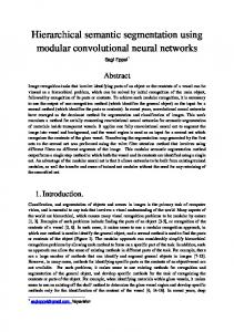
Fig. 1.

An example of hierarchical video segmentation obtained by our proposed method

Abstract—Hierarchical video segmentation provides regionoriented scale-space, i.e., a set of video segmentations at different detail levels in which the segmentations at finer levels are nested with respect to those at coarser levels. Hierarchical methods have the interesting property of preserving spatial and neighboring information among segmented regions. Here, we transform the hierarchical video segmentation into a graph partitioning problem in which each part will correspond to one region of the video. Thus, we propose a new methodology for hierarchical video segmentation which computes a hierarchy of partitions by a reweighting of original graph in which a segmentation can be easily infered. The temporal coherence is given, only, by color information instead of more complex features. We provide an extensive comparative analysis, considering both quantitative and qualitative assessments showing efficiency, ease of use, and temporal coherence of our methods. According to our experiments, the hierarchy infered by our two methods, p-HOScale and cp-HOScale, produces good quantitative and qualitative results when applied to video segmentation. Moreover, unlike other tested methods, our methods are not influenced by the number of supervoxels to be computed, as shown in the experimental analysis, and present a low space cost. Keywords-Hierarchical video segmentation; Edge-weighted graph; Partition; Observation scale.

I. I NTRODUCTION Image segmentation is the process of grouping perceptually similar pixels into regions. A hierarchical image segmentation is a set of image segmentations at different detail levels in which the segmentations at coarser detail levels can be produced from simple merges of regions from segmentations at

finer detail levels. Therefore, the segmentations at finer levels are nested with respect to those at coarser levels. Hierarchical methods have the interesting property of preserving spatial and neighboring information among segmented regions. Hierarchical video segmentation generalizes these concepts in order to consider spatiotemporal regions exhibiting in both appearance and motion. According to [1], the three major challenges for developing methods of video segmentation comprise: (i) temporal coherence; (ii) automatic processing; and (iii) scalabity. Nevertheless, hierarchical video segmentation methods cope very well with these challenges. However, some methods for video segmentation, such as those presented in [2] ignore temporal coherence. On the other hand, several video segmentation methods, such as the ones in [1], [3], [4], [5], may be considered as image segmentation extensions, in which the inclusion of temporal coherence (according to criteria of intensity, color and texture) is not a trivial task. Usually, methods for preserving temporal coherence will identify spatiotemporal video segments which are represented by supervoxels. In this work, the hierarchical video segmentation is transformed into a graph partitioning problem in which each part will correspond to one region of the video. Thus, a new methodology for hierarchical video segmentation is proposed which computes a hierarchy of partitions by a reweighting of the original graph in which a segmentation can be easily infered, and the temporal coherence is related to the graph transformation used, which, in this case, will consider only

color information. In Fig. 2, we illustrate the main steps of our methodology: (i) graph creation; (ii) computation of hierarchical scales; and (iii) inference of a video segmentation using thresholding. Any hierarchy can be represented by a tree, specially, a minimum spanning tree. The first appearance of this tree in pattern recognition dates back to the seminal work of Zahn [6]. Lately, its use for image segmentation was introduced by Morris et al. [7] in 1986 and popularized in 2004 by Felzenszwalb and Huttenlocher [8]. In [9], [10], the authors studied some optimality properties of hierarchical segmentations. Considering that, for a given image, one can tune the parameters of the well-known method proposed in [8] for obtaining a reasonable segmentation of this image. According to [8], the main parameter k is named as the observation scale. However, the region-merging method [8] does not provide a hierarchy and, consequently, it faces two major issues: • first, the number of regions may increase when the value of parameter k increases. This should not be possible if k was a true scale of observation: indeed, it violates the causality principle of multi-scale analysis, which states that a contour present at a scale k1 should be present at any scale k2 < k1 [11]; • second, even when the number of regions decreases, contours are not stable: they can move when the value of parameter k varies, violating the location principle. Following [11], we believe that, in order for the parameter k to be a true observation scale, we have to satisfy both the causality principle and the location principle, which leads to work with a hierarchy of segmentations. In [12], it is proposed the first algorithm to produce a hierarchy of segmentations based on region-merging method [8]. However, this method is an iterative version of the one proposed in [8] that uses a threshold function, and requires the tuning of a threshold parameter. The methods based on Nystrom [4] and segmentation by weighted aggregation (so-called SWA) [5], [13], both optimize the same normalized cut criterion. In [4], the Nystrom approximation was proposed to solve the eigenproblem, showing that it is possible to use this method for relatively low-resolution and short videos. The approach based on SWA proposed by [5], [13] computes iteratively the hierarchy considering for high hierarchical levels the previous ones. Moreover, it used an algebraic multigrid solver to efficiently compute the hierarchy. The mean shift segmentation (so-called MeanShift) which was proposed in [14] for image segmentation, it was applied to temporal sequences in [3]. Moreover, this work also introduced the Morse theory to interpret mean shift as a topological decomposition of the feature space into density modes. A hierarchical video segmentation is created by using topological persistence. For video segmentation, the method proposed by [1] (socalled GBH) taking into account the same criterium of [8] (socalled GB) iteratively computes different hierarchical levels, using an adjacency region graph. The first step of this method is to compute an oversegmented image that will be used as

first level of the hierarchy. It then iteratively constructs a region graph over the obtained segmentation, and forms a bottom-up hierarchical tree structure of the region (segmentation) graphs, unlike [8], the regions are described by local Lab histograms. To compute each hierarchical level, an edge-weighted graph is created in which the weights are the distance between the Lab histograms of the connected regions. Even though this method presents high quality segmentations with a good temporal coherence and with stable region boundaries, for computing a video segmentation according to a specified level, it is necessary to compute all lower (finer) segmentations. Here, we consider that when the scales increase the number of supervoxels decreases. Moreover, since Felzenszwalb and Huttenlocher’s method [8] is not hierarchical, some regions may be merged (as illustrated in [15]) and some computer vision operations may become too difficult. Following [15], in this paper, we provide a hierarchical version of the method proposed by Felzenszwalb and Huttenlocher applied to the hierarchical video segmentation that removes the need for parameter tuning and for the computation of video segmentation at finer levels. In other words, the proposed video segmentation is not dependent on the hierarchical level, and consequently, it is possible to compute any level without computing the previous ones, thus the time for computing a segmentation is almost the same for any specifed level (as will be shown at the experimental analysis). Contributions. The main result of this paper is an efficient hierarchical video segmentation algorithm based on the dissimilarity measure proposed in [8]. Our algorithm has a computational time cost similar to [1] and lower computational space cost, regarding the same problem, but it provides all scales of observations instead of only one segmentation level. Since it is a hierarchical method, its result satisfies both the locality principle and the causality principle. Namely in our approach, and in contrast to what happens with [8], the number of regions decreases when the scale parameter increases, and the contours do not move from one scale to another, and unlike the results of [1], it is not dependent on the first segmentation. This work is organized as follows. Section II presents fundamental concepts that are useful to this work and to some related works. In Section III, our approach for hierarchical video segmentation is presented along with simple examples to better explain how it really works. Then, experimental results are presented in Section IV together with a detailed quantitative and qualitative analysis. Finally, Section V presents final remarks and discusses possible research lines for future works. II. S OME FUNDAMENTAL CONCEPTS First, we define a supervoxel according to [16]. Given a 3D lattice Λ3 (the voxels in the video), a supervoxel sv is a subset of the lattice sv ⊂ Λ3 such that the union of all supervoxels S comprises the lattice and they are pairwise disjoint: i sv = T Λ3 and svi svj = ∅, ∀i, j pairs. Let V be a set. We denote by P(V ) the set of all subsets of V . Let x be an element of V and Px (V ) be the set of all subsets of V which contains the element x. A subset P ⊆

1

2

3

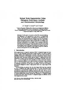
Fig. 2. Outline of our method. The method can be divided in three main steps: in step 1, the video is transformed into a video graph; in step 2, the hierarchy is computed from the video graph; and finally, in step 3, the identification of video segments is made from hierarchy.

P(V ) is called a partition (of V ) if the intersection of any two distinct elements of P is empty and if the union of all elements in P is equal to V . If P is a partition, each element of P is called a region (or class) of P. The set of all partitions of V is denoted by ΠV . Let P and P0 be two partitions of V . We say that P0 is a refinement of P if any region of P0 is included in a region of P. A set H = {Pλ ∈ ΠV | λ ∈ N} of (indexed) partitions is called a (indexed) hierarchy if for any two positive integers λ1 and λ2 such that λ1 ≥ λ2 , the partition Pλ2 is a refinement of Pλ1 . We define a (undirected) graph as a pair G = (V, E) where V is a finite set and E is composed of unordered pairs of V , i.e., E is a subset of {{x, y} ⊆ V | x 6= y}. Each element of V is called a vertex or a point of G, and each element of E is called an edge of G. A (simple) path in a graph is a sequence of edges which connects a sequence of vertices. A graph is said to be connected if every pair of vertices in the graph is connected. An edge-weighted graph is a pair W = (G, w) where G is a graph and w is a map from E(G) into N. A tree is a graph T = (V, E) which is connected and has only |V | − 1 edges. A spanning tree of a connected, undirected graph G = (V, E) is a tree T = (V 0 , E 0 ) in which V 0 = V and E 0 ⊆ E. For an edge-weighted graph W = (G, w) one associates an edge-weighted spanning tree U = (T, w) in which T is a spanning tree and w is a map from E(T ) into N. This map could be used to assign a weight to a spanning tree by computing the sum of the weights of all edges in that spanning tree. A minimum spanning tree (MST) (or minimum weight spanning tree) is then a spanning tree with weight less than or equal to the weight of every other spanning tree. Let us remember some definitions of region-merging criterion. The criterion for region-merging in [8] measures the evidence for a boundary between two regions by comparing two quantities: one based on intensity differences across the boundary, and the other based on intensity differences between neighboring pixels within each region. More precisely, in order to know whether two regions must be merged, two measures are considered. The internal difference Int(X) of a region X is the highest edge weight among all the edges linking two vertices of X in the MST. The difference Diff (X, Y ) between

two neighboring regions X and Y is the smallest edge weight among all the edges that link X to Y . Then, two regions X and Y are merged when: Diff (X, Y ) ≤ min{Int(X) +

k k , Int(Y ) + } |X| |Y |

(1)

where k is a parameter used to prevent the merging of large regions (i.e., larger k forces smaller regions to be merged). The merging criterion defined by Eq. (1) depends on the scale k at which the regions X and Y are observed. More precisely, let us consider the (observation) scale SY (X) of X relative to Y as a measure based on the difference between X and Y , on the internal difference of X and on the size |X| of X: SY (X) = (Diff (X, Y ) − Int(X)) × |X|.

(2)

Then, the scale S(X, Y ) is simply defined as: S(X, Y ) = max(SY (X), SX (Y )).

(3)

Thanks to this notion of a scale, Eq. (1) can be written as: k ≥ S(X, Y ).

(4)

Let T = (V, E) be a tree and U = (T, w) an edge-weighted tree. Let PV be a partition of V and let X be a region of PV . The internal difference of X in U , denoted by Int U (X), is the highest weight of an edge in E(T ) that links two elements of X (i.e., Int U (X) = max{w({x, y}) | {x, y} ∈ E(T ), x ∈ X, y ∈ X}). Let Y be another region of P. We say that X and Y are two adjacent regions if there exists an edge {x, y} of T such that x belongs to X and y belongs to Y ; in this case, we also say that the edge {x, y} links X and Y . If X and Y are adjacent, the difference between X and Y – Diff U (X,Y) – is the lowest weight of an edge that links X and Y . Furthermore, if X and Y are adjacent, the (observation) scale SYU (X) of X relative to Y in U is given by SYU (X) = (Diff U (X, Y ) − Int U (X)) × |X| and the scale of X and Y in U , denoted by S U (X, Y ), is given U (Y )). by S U (X, Y ) = max(SYU (X), SX

X

Y

X

Y

10

18

B

4 H

9 A

15 E

2 10 C

6

G

9

15 1

B

G

1 8

F

1 10

14

(a)

12

A E

2

1 D

H

21

I

C

1

F

1 D

I

(b)

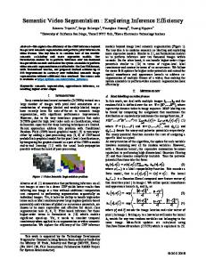
Fig. 3. Example for computing the hierarchical scale for an edge-weighted graph. For this example, we suppose that all scales for the regions X and Y are already computed, and we will calculate the hierarchical scale for the edge connecting B and G.

III. A HIERARCHICAL VIDEO SEGMENTATION METHOD weights. 0 (ii) Let PV = {{vi } | vi ∈ V 0 } Our method for hierarchical video segmentation, illustrated in Fig. 2, is based on computation of (hierarchical) obser- (iii) Let x and y be two vertices of V that are connected by i-th non evaluated edge e in the ordering. vation scales between any two adjacent regions. Following 0 (iv) Find the region X of PV that contains x. [8], instead of computing these scales directly from the video, 0 V our approach computes them on a graph generated from the (v) Find the region Y of P that contains y. video. Note that the modeling used to transform the video into (vi) Compute the hierarchical observation scale an edge-weighted graph may influence the calculation of the we0 = max{SY (X), SX (Y )} scales (Step 1 in Fig. 2), and, consequently, it may modify the edge e0 = (x, y) into E 0 and add we0 to the edge results that will be obtained by our method (as will be dis- (vii) Insert an 0 map w associated with the new edge e0 . cussed in more detail in Section IV). In this section, we focus V0 V0 the discussion over the process for computing the hierarchical (viii) Let P = P \ {X, Y } ∪ {Z | Z ∈ X ∪ Y } scales from video graph (Step 2 in Fig. 2). This approach is (ix) Repeat the steps (iii)-(viii) until there is no edge left. b) Algorithm 2: Compute observation scale of a region similar to the one proposed for image segmentation by [15], that contains x relative to Y – SY (X). Here, we consider the in which the adjacent regions that are evaluated depend on edge-weighted tree U = (T, w) and the edge-weighted graph the order of the merging in the fusion tree (or simply, the 0 0 0 U = (G , w ) as defined in Algorithm 1. order of the connected component merging on the minimum I 0 0 spanning tree of the original graph). As will be seen later, a (1) Let Px (V ) ⊆ Px (V ) be the set of all subsets of 0 V which contains the element x in which each subset new edge-weighted tree is created from the MST in which induces a connected graph. each edge weight corresponds to the scale from which two I 0 adjacent regions connected by this edge are correctly merged, (2) Find the largest set, X0 ∈ Px (V ), in terms of size, in U U which SY (X) ≥ Int (X), i.e. i.e., there are no two sub-regions of these regions that might 0 be merged before these regions. In fact, instead of computing SYU (X) ≥ Int U (X) and | X | ≥ | X 0 |, ∀X, X 0 ∈ PxI (V 0 ) the hierarchy of partitions, a weight map is produced from which the desired hierarchy can be inferred (Step 3 in Fig. 2), (3) Compute C = {Ci ∈ PxI (V 0 ) | X ⊂ Ci }. SY (X) = SYU (X) else SY (X) = e.g., by removing from those edges whose weight is greater (4) If C = ∅ then U0 than the desired scale. min{min{Int (Ci ) | Ci ∈ C}, SYU (X)}. Our method described by Algorithm 1 (hereafter called (5) Return SY (X). HOScale) for computing the weight map is based on the We will explain the steps of our algorithms using an analysis of a fusion tree oriented by merging of regions example. Let us illustrate the computation of a hierarchical according to non-decreasing edge weight, i.e., the MST of observation scale on the graph of Fig. 3(a). To this end, we original graph is used for orienting these fusions. The kernel of consider the iteration of the algorithm at which the edge e our methodology is presented in Algorithm 2, since it identifies linking B to G is analyzed. At this step, the edges of the the smaller scale value that can be used to merge the largest MST of weight below w(e) = 10 have been already processed. region to another region while guaranteeing that the internal Therefore, the hierarchical observation scale of these edges differences of these merged regions are larger than the value (depicted by continuous lines in the figure) is already known calculated for the smaller scale. as shown in Fig. 3(b). The regions X and Y obtained at a) Algorithm 1: Compute the observation scale between Steps (iv) and (v) are set to {A, B, C, D, E} and {F, G, H, I} X and Y . Let T = (V, E) be a tree. Let G = (V 0 , E 0 ) be respectively. Then, in order to find the value we0 at Step (vi) a graph, in which V 0 = V and E 0 = ∅. Let U = (T, w) be of the Algorithm 1, all partitions (for each region) must be an edge-weighted tree. Let U 0 = (G, w0 ) be an edge-weighted considered. graph. Firstly, let us analyse the region X of Fig. 3(b). The (i) Sort E(T ) into π = (o1 , · · · , om ) by non-decreasing edge set of all subsets of X which contains the element x and

To efficiently implement our methods, we use some data structures similar to the ones proposed in [15]; in particular, the management of the collection of partitions is made using Tarjan’s union-find and Fredman and Tarjan’s Fibonnacci heaps. Furthermore, we made some algorithmic optimizations to speed up the computations of the hierarchical observation scales. So, in order to create the video graphs, and when it is necessary, we employ a KD-tree for identifying the K-nearest neighbors. Our method is implemented in C++. We ran all experiments in a Quad-Core Intel Xeon E5620 2.4Ghz 24GB RAM with Ubuntu 12.04.1 LTS. Regarding computational cost, both methods, p-HOScale and cp-HOScale, outperform all tested methods in space cost (as illustrated in Fig. 4). This metric is important if we consider applications in environments without enough RAM memory, like ultrabooks. For example, we do not plot SWA information since, according to our experiments, it consumes about 45 GB for a video with 100 frames. B. Quantitative analysis Using the library LIBSVX, developed by [16], it is possible to compute, among others, the following metrics: (i) 3D boundary recall; (ii) 3D segmentation accuracy; (iii) 3D undersegmentation errors; (iv) explained variation; and (v) mean duration. The 3D boundary recall assesses the quality of the spatiotemporal boundary detection, while the 3D segmentation accuracy quantifies what fraction of groundtruth 3

400

2.8 2.6 2.4

350

cp-HOScale

250

300

Time (s)

2.2

GB GBH p-HOScale

2 1.8

GB GBH

200

p-HOScale cp-HOScale

150

1.6 100 1.4 50

1.2 1 200

300

400

500

600

700

800

0 200

900

300

Number of Supervoxels

400

500

600

700

800

900

Number of Supervoxels

(a) 4

500 450

GB GBH p-HOScale

3.5

3

400 350

cp-HOScale Time (s)

In order to provide a comparative analysis, we take into account the benchmark and library LIBSVX proposed in [16], since the implemented methods are the state of the art for early hierarchical video segmentation. The benchmark is composed, among others, by: • two datasets with groundtruth - Chen Xiph.org [17], SegTrack [18]. The Chen’s dataset Xiph.org is composed by eight videos which are densely labeled, with an average of 85 frames-per-video (fpv), a minimum of 69 fpv and a maximum of 86 fpv, leading to a total of 639 annotated frames. The dataset SegTrack is composed by six videos, with an average of 41 fpv, a minimum of 21 fpv and a maximum of 71 fpv, leading to a total of 244 annotated frames. It is important to note that the groundtruth of the second dataset, SegTrack, is composed by only one segmented object. Moreover, the video databases are not splitted into training/testing data sets; • implementations of the methods GB ([8]), GBH ([1]), MeanShift ([3]), Nystrom ([4]) and SWA ([13]) applied to video segmentation. As can be seen in Fig. 2 and discussed at the beginning of Section III, the method HOScale computes a new weight map from a video graph, however there are several ways for transforming a video into a video graph. Here, we will consider only two: • the underlying graph is the one induced by the 26-adjacency pixel relationship, where the edges are weighted by a simple color gradient computed by the Euclidean distance in the RGB space, so this method is called p-HOScale (where p stands for pixel relationship); • the underlying graph is the one induced by the 26adjacency pixel relationship together with the 10 nearest neighbors in RGBXYZ space, where the edges are again weighted by a simple color gradient computed by the Euclidean distance in the RGB space, this method is

A. Implementation issues

Memory (GB)

IV. E XPERIMENTAL ANALYSIS

called cp-HOScale (where c and p stand for color and pixel relationship, respectively). The GTech dataset [1] is also used in our qualitative analysis. Moreover, in our experiments, we consider the real size of the videos, in terms of frame size, instead of rescaling (as proposed in [16]).

Memory (GB)

the induced graph has only 1 (one) connected component which is PxI (V 0 ) = {{B}, {B, C}, {A, B, C, D, E}}. In Step 2 (Algorithm 2), we look for the largest set in which the hierarchical observation scale is greater than or equal to the internal difference of the new re-weighted tree. Thus, suppose that X = {A, B, C, D, E}, as SYU (X) = (10 − 9) × 5 = 5 0 is smaller than Int U (X) = 21 (which is the highest edge weight of X), then it is necessary to verify for another set. Now, for X = {B, C}, the SYU (X) = (10 − 1) × 2 = 18 is 0 greater than or equal to Int U (X) = 1, then SY (X) = 18, which is the minimum between 18 and 21 (steps 3 and 4 of Algorithm 2). The same process is made for SX (Y ). The set of all subsets of Y which contains the element y and the induced graph has only 1 (one) connected component, which is PyI (V 0 ) = {{G}, {G, H, I}, {F, G, H, I}}, here SX (Y ) = 12, which is the minimum between 12 and 18. Finally, the hierarchical observation scale of X and Y is 18 (= max{SY (X), SX (Y )} = max{18, 12}).

2.5

2

GB 300

GBH p-HOScale

250

cp-HOScale 200 150

1.5 100 1 200

300

400

500

600

700

800

900

Number of Supervoxels

50 200

300

400

500

600

700

800

900

Number of Supervoxels

(b) Fig. 4. A comparison between our methods, p-HOScale and cp-HOScale, and the methods GB and GBH when applied to Chen’s (a) and SegTrack (b) datasets. The comparison is based on the following metrics (from left to right): (i) space cost; (ii) total time for all methods.

1

0.9

0.8

0.8

0.8

0.7

0.6

SWA GB GBH Meanshift Nystr¨o m p-HOScale cp-HOScale

0.5

0.4

300

400

500

600

700

800

0.7

0.6

SWA GB GBH Meanshift Nystr¨o m p-HOScale cp-HOScale

0.5

0.4

0.3 200

900

300

Number of Supervoxels

500

600

700

SWA GB GBH Meanshift Nystr¨o m p-HOScale cp-HOScale

0.3 200

900

60 50 40 30

500

600

700

800

900

600

700

0.7

0.6

0.4 200

800

900

SWA GB GBH Meanshift Nystr¨o m p-HOScale cp-HOScale

60

SWA GB GBH Meanshift Nystr¨o m p-HOScale cp-HOScale

10

Number of Supervoxels

500

Number of Supervoxels

0.8

0.5

400

400

65

20

300

300

70

0.9

Explained Variation

70

SWA GB GBH Meanshift Nystr¨o m p-HOScale cp-HOScale

0.4

1

80

0 200

800

0.6

Number of Supervoxels

90

3D Undersegmentation Error

400

0.7

0.5

Mean Duration

0.3 200

3D F−measure

1

0.9

3D Boundary Recall

3D Segmentation Accuracy

1

0.9

300

400

500

600

700

800

55

50

45

40

900

35 200

Number of Supervoxels

300

400

500

600

700

800

900

Number of Supervoxels

Fig. 5. A comparison between our methods, p-HOScale and cp-HOScale, and the methods GB, GBH, SWA, MeanShift and Nystrom when applied to Chen’s dataset. The comparison is based on the following metrics: (i) 3D segmentation accuracy; (ii) 3D boundary recall; (iii) 3D F-measure; (iv) 3D undersegmentation error; (v) explained variation and (vi) mean duration.

segments is correctly classified. The 3D undersegmentation error measures what fraction of voxels exceeds the volume boundary of the groundtruth region and the explained variation is a human independent measure assessing spatiotemporal uniformity. Finally, the mean duration quantifies the average duration, in terms of number of frames, of the video segments (or supervoxels). Here, we also compute a 3D F-measure which is a harmonic mean that measures how good is a segmentation regarding both 3D boundary recall and 3D segmentation accuracy. Fig. 5 and Fig. 6 illustrate the average values of computed metrics for Chen’s dataset and SegTrack dataset varying the number of desired supervoxels between 200 and 900, in which the parameters for our methods are tunned per dataset, like in GB, SWA and Meanshift, exporting out the best obtained results. For GB and Nystrom, the parameters are tunned per video. The strategy for filtering out small regions is the same adopted in [16], in which the size of the regions to be filtered out increases, by a constant value, when the number of supervoxels decreases. Note that, unlike GBH, SWA and MeanShift, our methods have an exact control on the desired number of video segments (or supervoxels). For the Chen’s dataset, we can observe that cp-HOScale presents similar results when compared to the best one (SWA for explained variation and GBH for another measures). For SegTrack dataset, the same behavior is observed except for mean duration in which cpHOScale ourperfoms the best one. According to [19], the mean duration of segments is a more important metric, as it measures the temporal coherence of a segmentation method more directly, and as one can see in Fig. 5 and Fig. 6, cpHOScale outperforms all other methods for SegTrack dataset,

and it is equivalent to the best one for Chen’s dataset. In both datasets, the 3D segmentation accuracy presents similar results with respect to GBH and SWA, however this metric is quite constant for all number of supervoxels, representing its stability. Considering total time, our methods outperform GBH when we compute a small number of video segments. As one can see, in Fig. 4, our methods have a constant time for computing any hierarchical level while GBH has an increasing time when the number of supervoxels decreases. Remember that the scales increase when the number of supervoxels decreases. It is important to note that the method p-HOScale, when compared to its non-hierarchical version GB, outperforms it for all metrics. Thus, it is not easy to conclude what method is better with respect to the others. However, we outperform the other methods (in different datasets) in several cases, and in the cases that our method (cp-HOScale) is not the best, it presents similar results to the best ones. Moreover, despite the initialization time of our method, the time for computing every segmentation is constant. C. Qualitative analysis Despite the quantitative results, we also compared visually some of the tested methods in order to illustrate the behavior when we varied the number of video segments (50 and 100) to be computed. In Fig. 7 and Fig. 8, we illustrate results obtained when we apply the methods GB, GBH, SWA, p-HOScale and cp-HOScale for videos extracted from GTech and Chen’s datasets, respectively. Note that, unlike cp-HOScale and pHOScale, there is no guarantee that the three other methods will obtain the specified number of video segments, thus we

1

0.9

0.8

0.8

0.8

0.7

0.6

SWA GB GBH Meanshift Nystr¨o m p-HOScale cp-HOScale

0.5

0.4

300

400

500

600

700

800

0.7

0.6

SWA GB GBH Meanshift Nystr¨o m p-HOScale cp-HOScale

0.5

0.4

0.3 200

900

300

Number of Supervoxels

500

600

700

SWA GB GBH Meanshift Nystr¨o m p-HOScale cp-HOScale

0.3 200

900

15

0.7 0.65

SWA GB GBH Meanshift Nystr¨o m p-HOScale cp-HOScale

0.6

10 0.5

500

600

700

800

600

700

900

0.45 200

800

900

SWA GB GBH Meanshift Nystr¨o m p-HOScale cp-HOScale

26

0.8 0.75

0.55

Number of Supervoxels

500

Number of Supervoxels

0.85

20

400

400

28

25

300

300

30

0.9

Explained Variation

30

SWA GB GBH Meanshift Nystr¨o m p-HOScale cp-HOScale

0.4

0.95

35

5 200

800

0.6

Number of Supervoxels

40

3D Undersegmentation Error

400

0.7

0.5

Mean Duration

0.3 200

3D F−measure

1

0.9

3D Boundary Recall

3D Segmentation Accuracy

1

0.9

300

400

500

600

700

800

24

22

20

18

900

16 200

300

Number of Supervoxels

400

500

600

700

800

900

Number of Supervoxels

Fig. 6. A comparison between our methods, p-HOScale and cp-HOScale, and the methods GB, GBH, SWA, MeanShift and Nystrom when applied to SegTrack dataset. The comparison is based on the following metrics:(i) 3D segmentation accuracy; (ii) 3D boundary recall; (iii) 3D F-measure; (iv) 3D undersegmentation error; (v) explained variation and (vi) mean duration.

(a)

(b)

Fig. 7. Examples of video segmentations for a video extracted of the GTech. The original frames are illustrated in the first row. The following rows, from top to bottom, illustrate the results obtained by GB, GBH, p-HOScale, cp-HOScale and SWA, respectively. The parameters were tunned to obtain about (a) 50 and (b) 100 video segments.

compute a segmentation containing a number of regions, as close as possible, for the specified threshold. Regarding the segmentation for each frame, we may observe that our methods present goods results when visually compared to the other methods. Moreover, cp-HOScale is subjectively better than p-HOScale. The same behavior may be observed for temporal coherence. Despite the good quantitative results obtained by SWA, its results are not visually as good as GBH and our methods.

V. C ONCLUSIONS AND F UTURE W ORKS In this work, we proposed a method for early hierarchical video segmentation based on computation of hierarchical observation scales. Our method can be divided into 3 (three) main steps: (i) graph creation; (ii) computation of hierarchical scales; and (iii) inference of video segmentation using thresholding. We studied two possibilities for producing the video graph in order to verify the influence of color and pixel location. To compute our hierarchical scales, we propose a methodology for reweighting the minimum spanning tree

(a)

(b)

Fig. 8. Examples of video segmentations for a video extracted of the Chen’s dataset. The original frames are illustrated in the first row. The following rows, from top to bottom, illustrate the results obtained by GB, GBH, p-HOScale, cp-HOScale and SWA, respectively. The parameters were tunned to obtain about (a) 50 and (b) 100 video segments.

computed from the video graph based on a criterion that measures the evidence for a boundary between two regions by comparing the intensity differences across the boundary and the intensity difference between neighboring voxels within each region. Finally, the partitioning of the graph, after the reweighting, is based on removing the edges whose weights (which represent the scales) are greater than or equal to a specified scale. Each graph region represents a video segment. According to our experiments, the hierarchies infered by our two methods, p-HOScale and cp-HOScale, produce good quantitative and qualitative results when applied to video segmentation. Moreover, unlike other tested methods, our methods are not influenced by the number of supervoxels to be computed, as shown in the experimental analysis, and present a low space cost. For further works, we will study different ways for computing the video graph, mainly, in order to decrease the time for its creation and assess its impact on video segmentation results. Moreover, we will study how to extend our method for streaming video segmentation. ACKNOWLEDGMENT The authors are grateful to PUC Minas, UFMG, ESIEE, CNPq, CAPES, COFECUB and FAPEMIG for the financial support of this work. R EFERENCES [1] M. Grundmann, V. Kwatra, M. Han, and I. Essa, “Efficient hierarchical graph based video segmentation,” in CVPR, 2010. [2] J. Chen, S. Paris, and F. Durand, “Real-time edge-aware image processing with the bilateral grid,” in ACM SIGGRAPH 2007 papers, ser. SIGGRAPH ’07. New York, NY, USA: ACM, 2007. [3] S. Paris and F. Durand, “A topological approach to hierarchical segmentation using mean shift,” in CVPR, 2007, pp. 1–8.

[4] C. Fowlkes, S. Belongie, and J. Malik, “Efficient spatiotemporal grouping using the nystrom method,” in CVPR, vol. 1, 2001, pp. I–231–I–238 vol.1. [5] J. Corso, E. Sharon, S. Dube, S. El-Saden, U. Sinha, and A. Yuille, “Efficient multilevel brain tumor segmentation with integrated bayesian model classification,” IEEE Transactions on Medical Imaging, vol. 27, no. 5, pp. 629–640, 2008. [6] C. T. Zahn, “Graph-theoretical methods for detecting and describing gestalt clusters,” IEEE Trans. Comput., vol. 20, pp. 68–86, January 1971. [7] O. Morris, M. J. Lee, and A. Constantinides, “Graph theory for image analysis: an approach based on the shortest spanning tree,” Communications, Radar and Signal Processing, IEE Proceedings F, vol. 133, no. 2, pp. 146 –152, april 1986. [8] P. F. Felzenszwalb and D. P. Huttenlocher, “Efficient graph-based image segmentation,” IJCV, vol. 59, pp. 167–181, September 2004. [9] L. Najman, “On the equivalence between hierarchical segmentations and ultrametric watersheds,” JMIV, vol. 40, pp. 231–247, 2011. [10] J. Cousty and L. Najman, “Incremental algorithm for hierarchical minimum spanning forests and saliency of watershed cuts,” in ISMM, ser. LNCS. Springer, 2011, vol. 6671, pp. 272–283. [11] L. Guigues, J. P. Cocquerez, and H. L. Men, “Scale-sets image analysis,” IJCV, vol. 68, no. 3, pp. 289–317, 2006. [12] Y. Haxhimusa and W. Kropatsch, “Segmentation graph hierarchies,” in SSPR/SPR. Springer, 2004, vol. 3138, pp. 343–351. [13] E. Sharon, A. Brandt, and R. Basri, “Fast multiscale image segmentation,” in CVPR, vol. 1, 2000, pp. 70–77 vol.1. [14] D. Comaniciu and P. Meer, “Mean shift: A robust approach toward feature space analysis,” IEEE Trans. Pattern Anal. Mach. Intell., vol. 24, no. 5, pp. 603–619, May 2002. [15] S. J. F. Guimarães, J. Cousty, Y. Kenmochi, and L. Najman, “A hierarchical image segmentation algorithm based on an observation scale,” in SSPR/SPR, 2012, pp. 116–125. [16] C. Xu and J. J. Corso, “Evaluation of super-voxel methods for early video processing,” in CVPR, 2012. [17] A. Y. C. Chen and J. Corso, “Propagating multi-class pixel labels throughout video frames,” in Proceedings of Western New York Image Processing Workshop, 2010. [18] D. Tsai, M. Flagg, and J. M.Rehg, “Motion coherent tracking with multilabel mrf optimization,” BMVC, 2010. [19] C. Xu, C. Xiong, and J. J. Corso, “Streaming hierarchical video segmentation,” in ECCV, 2012.