The integration of inertial sensors with a camera allows exploiting the better .... (s1,s2,s3)T . A vector is sometimes regarded as a column matrix. So vector ...
High Altitude UAV Navigation using IMU, GPS and Camera Cesario Vincenzo Angelino, Vincenzo Rosario Baraniello, Luca Cicala CIRA, the Italian Aerospace Research Centre Capua, Italy Email: {c.angelino,v.baraniello,l.cicala}@cira.it Abstract—This paper deals with the integration of measurements provided by inertial sensors (gyroscopes and accelerometers), GPS (Global Positioning System) and a video system in order to estimate position and attitude of an high altitude UAV (Unmanned Aerial Vehicle). In such a case, the vision algorithms present ambiguities due to the plane degeneracy. This ambiguity can be avoided fusing the video information with inertial sensors measurements. On the other hand, inertial sensors are widely used for aircraft navigation because they represent a low cost and compact solution, but their measurements suffer of several errors which cause a rapid divergence of position and attitude estimates. To avoid divergence, inertial sensors are usually coupled with other systems as for example GPS. A camera presents several advantages with respect to GPS as for example great accuracy and higher data rate. Moreover, it can be used in urban area or, more in general, where no useful GPS signal is present. On the contrary, it has lower data rate than inertial sensors and its measurements have latencies which can prejudice the performances and the effectiveness of the flight control system. The integration of inertial sensors with a camera allows exploiting the better features of both the systems, providing better performances in position and attitude estimation. The data fusion is performed via a multirate Unscented Kalman Filter (UKF) because of the nonlinear dynamic system equation. Experimental results show the effectiveness of the proposed method.
I.
I NTRODUCTION
UAV navigation based on vision algorithms is still a challenging problem. One of the main challenges is when the scene points are situated on a plane. This is rather typical for a UAV to fly at a high altitude such that the earth surface can be approximated with a plane or, in addition, to cases where the UAV is flying over a naturally planar field. In this cases the vision based ego motion estimation is ambiguous. A promising way to overcome this ambiguity is the integration of video systems (VS) with measurements provided by inertial sensors (gyroscopes and accelerometers) [1]. Indeed these kind of sensors bring complementary chacacteristics. Inertial sensors are widely used for aircraft navigation because they represent a low cost and compact solution, but their measurements suffer of several errors which cause a rapid divergence of position and attitude estimates. To avoid divergence, inertial sensors are usually coupled with other systems as for example GPS. On the other hand, a camera is generally installed on-board UAVs for surveillance purposes, it presents several advantages with respect to GPS as for example great accuracy and higher data rate. Moreover, it can be used in urban area or, more in general, where multipath effects can forbid the application of GPS. A camera, coupled with a video
processing system, can provide attitude and position (up to a scale factor), but it has lower data rate than inertial sensors and its measurements have latencies which can prejudice the performances and the effectiveness of the flight control system.The integration of inertial sensors with a camera allows exploiting the better features of both the systems, providing better performances in position and attitude estimation. There are two broad approaches for integration of vision and inertial sensing, usually called loosely and tightly coupled. The loosely coupled approach uses separate INS and VS blocks, running at different rates and exchanging information. The tightlycoupled systems combine the disparate raw data of vision and inertial sensors in a single, optimum filter, rather than cascading two filters, one for each sensor. Tipically, in order to fusion the data a Kalman Filter is used. The use of inertial sensors in machine vision applications has been proposed by now more than twenty years ago and further studies have investigated the cooperation between inertial and visual systems in autonomous navigation of mobile robots, in image correction and to improve motion estimation for 3D reconstruction of structures. More recently, a framework for cooperation between vision sensors and inertial sensors has been proposed. The use of gravity as a vertical reference allows the calibration of focal length camera with a single vanishing point, the segmentation of the vertical and the horizontal plane. In [2] is presented with a function for detecting the vertical (gravity) and 3D mapping, and in [3] such vertical inertial reference is used to improve the alignment and registration of the depth map. Applications in robotics are increasing. Initial works on vision systems for automated passenger vehicles have also incorporated inertial sensors and have explored the benefits of visual-inertial tracking [4], [5]. Other applications include agricultural vehicles [6], wheelchairs [7] and robots in indoor environments [8], [9]. Other recent work related to Unmanned Aerial Vehicles (UAV) include fixedwing aircraft [10], [11], [12], [13], rotorcraft [14], [15] and spacecraft [16]. For underwater vehicles (AUVs) recent results can be found in [17], [18], [19]. A good overview of the methods applied for attitude estimation using a video system is provided in [20]. These methods can be generally distinguished in: a) methods based on horizon detection, b) methods based on the analysis of the optical flow, c) methods based on the detection of salient features in the field of view. In [21] the pitch and roll angles, and three body angular rates are determined by detection of the horizon in a sequence of images and by the analysis of the optical flow. The use of the horizon detection technique
does not allow determining the value of the yaw angle, whose knowledge is required, for example, in trajectory tracking algorithms. Moreover, for some configurations of the video system or particular maneuvers, the horizon could not be present in the images (for example cameras could frame only the sky if they are also used for Collision Avoidance). In [22] it is proposed another method, based on the detection of the horizon in an images sequence, to estimate roll and pitch angles. In [23] the aircraft complete attitude is determined using a single camera observations. Specifically, the proposed method required the knowledge of the positions of the own aircraft and of the points identified in the camera images. (a georeferenced map of the surrounding space is required). In [24] it is proposed another method to estimate both aircraft position and attitude using a single camera. In this application is required the presence of some reference points or some known geometries in the surrounding space too. This paper is organized as follow. In Section II some notations are introduced. Section III provides a description of the camera system. Section IV and Section V deal with the estimation of camera egomotion and the Kalman Filtering respectively. Experimental setup and numerical analysis are described in Section VI. Finally, conclusions are drawn in Section VII. II.
N OTATIONS
We first introduce some notation. Matrices are denoted by capital italics. Vectors are denoted by bold fonts either capital or small. A three-dimensional column vector is specified by (s1 , s2 , s3 )T . A vector is sometimes regarded as a column matrix. So vector operation such as cross product (×) and matrix operations such as matrix multiplication are applied to three-dimensional vectors. Matrix operations precede vector operations. 0 denotes a zero vector. For a matrix A = [aij ], ||A|| denotes the Euclidean norm of the matrix, i.e., ||[aij ]|| = q P 2 ij aij . We define a mapping [·]× from a three-dimensional vector to a 3 by 3 matrix: " # 0 −x3 0 � � T x3 0 −x1 . (x1 , x2 , x3 ) × = (1) −x2 x1 0 Using this mapping, we can express cross operation of two vectors by the matrix multiplication of a 3 by 3 matrix and a column matrix: X × Y = [X]× Y. (2) The reference system s, in which the coordinates of the vector x are expressed, is reported as superscribe on the upper-left corner of x with the notation xs . The reference systems considered in the paper are the following: i e n b c
inertial system; the ECEF (Earth Cenetered Earth Fixed) system; the NED (North East Down) system, tangent to the earth ellipsoid, at a reference Latitude and Longitude (Lat0 , Lat0 ); the ”body” system as seen by the IMU (Inertial Measurement Unit); the camera system, with fixed orientation with respect the IMU.
Fig. 1.
Homography inducted by the plane Π.
III.
P LANAR UAV E GO - MOTION
A. Coordinate System The default coordinate system in which the UAV position, i.e. (Lat, Lon, Alt) of the vehicle center of mass, is given is the ECEF system. Cne is the reference change matrix from NED to ECEF. The attitude and heading of the vehicle is given as Cbn (φ, θ, ψ) where Cbn is the reference change matrix associated with the roll (φ), pitch (θ), and yaw (ψ) angles. In general, the camera standard reference system might be rotated with respect to the body reference system. Thus, the transformation from the camera reference to ECEF is given by Cce = Cne (Lat, Lon) Cbn (φ, θ, ψ) Ccb
(3)
Ccb
represents the constant reference change matrix from where camera system c to body unit system b. B. Homography Matrix Let us consider a 2-D plane Π in 3-D space as in Figure 1. Consider two images taken by the camera at different time. The equation linking two image points p0 and p which are the projection of the same point of Π is: p0 ' HΠ p,
(4)
where p0 = [u0 , v 0 , 1]T and p = [u, v, 1]T are the (normalized) homogeneous coordinates in the second and the first camera reference frame respectively and the symbol ' means that equality is up to a scale factor. We call the matrix � c2 T � r21 N c2 (5) HΠ = Cc1 + d the planar homography matrix induced by the plane� Π. It con� c2 tains the information about the camera movement ( Ccc12 , r21 ) ant the scene structure (the normal to the plane N, and the distance d). We suppose that the scene structure is known from the GPS position and � � the terrain digital elevation model c2 (DEM). Here Ccc12 , r21 represents the rigid transformation (rotation and translation) which brings points (i. e. transforms coordinates) from the camera 1 to the camera 2 standard reference system. The coordinates change equation is given by c2 (6) xc2 = Ccc12 xc1 + r21 where xck represent the coordinates in the camera k standard reference system.
s The translation vector between the two camera center r12 = O2s − O1s expressed in a generic reference system s is equal to c2 −C2s r21 . The matrix Ccc12 contains in it different contributions:
1)
the rotation of the camera by the pan-tilt unit;
2)
changes in the vehicle attitude and heading;
3)
rotation between the two NED systems (in t2 and t1 ).
Indeed it can be also expressed as Ccc12 = Cec2 Cce1 = Cce2 T Cce1
(7)
By means of eq. (3) and with a little algebra we obtain c2 Ccc12 = Cb2 Cnb22 Cen2 Cne 1 Cbn11 Ccb11 | {z }
(8)
≈I
In the above equation we supposed (Lat,Lon) did not change a lot between two consecutive frames, hence the idendity approximation. This also means that the two NED reference systems (i.e., corresponding to n1 and n2 ) can be thought to be coincident up to a translation. The eq.(8) then reads as Ccc12 ≈ Cbc22 Cnb22 Cbn11 Ccb11 .
(9)
Therefore, supposing a fixed camera orientation with respect to the body, the functional dependency is only in the rotation of the body, i.e. in the change of the vehicle attitude and heading, Cbb12 ≈ Cnb22 Cbn11 ≈ R(dφ, dθ, dψ) = Rx (dφ)Ry (dθ)Rz (dψ) (10) where dφ = φ2 − φ1 , dθ = θ2 − θ1 and dψ = ψ2 − ψ1 . The expression of R is given in (11) on the top of the next page. It can be approximated for small angle variations by ! 1 dψ −dθ −dψ 1 dφ R(dφ, dθ, dψ) ≈ = I − Ωb dt (12) dθ −dφ 1 where ω b = [dφ, dθ, dψ]T /dt is the angular velocity of the b system with respect to n in the body reference system and Ωb = [ω b ]× . c2 r21
Ccc12
Once estimated and from the homography matrix H, they give information on v(t) and ω(t) respectively. Such an information can be used either as a prediction or as a measurement for the Kalman Filter. Similarly, the IMU output can be used as a priori information for the vision algorithms. IV.
C OMPUTATION OF H AND MOTION ESTIMATION
A. Fast computation of image point corrispondences To calculate the homography matrix by video analysis, the point correspondences between two successive frames can be calculated using a computer vision system based on the Lukas-Kanade method [25]. This method assumes that the displacements of the points belonging to the image plane is small and approximately constant. Thus the velocity of the points in the image plane must satisfy the Optical Flow equation ˙ Iu (p)u˙ + Iv (p)v˙ = −I(p), (13) where p = (u, v) is a point in the image plane, Iu , Iv are the components of the spatial gradient of the image intensity in the
image plane and x˙ is the notation for the temporal derivative of x. The Lucas-Kanade method [25] can be used only when the image flow vector between the two frames is small enough for the differential equation of the optical flow to hold. When this condition does not hold, a rough preliminary prediction of the optical flow must be performed with other methods and the Lukas-Kanade method can be used for refinement only. When external sensors, like IMU or GPS (Global Positioning System), are available, the camera motion is predictable, so that a rough estimation of the optical flow can be easily initialized starting from the sensor measurements [26]. To aim this task, a basic knowledge of the scene 3D geometry should be known or at least approximatively known. This is the case of the Earth surface that can be modeled as ellipsoid, geoid or digital elevation model. Using this prior information, the computational burden of the optical flow estimation can be strongly reduced, so that the delay of the video processing can be made compatible with the application of the proposed technology of sensor fusion to the navigation scenario. To further reduce the computational burden of the computer vision algorithms an improvement of the Lukas-Kanade method, the Kanade-Lucas-Tomasi (KLT) feature matching algorithm [27], has been adopted. The KLT has been improved using the ellipsoid model of the Earth surface, increasing the speed of calculus of the Optical Flow. B. Homography matrix calculation Obtained a set of correspondences of coplanar points for a couple of successive frames, our objective is to find the homography matrix HΠ such as Eq. (4) holds. An example of candidate points for homography estimation is given in Figure 2. Let " # h1 h4 h7 HΠ = h2 h5 h8 , hS = (h1 , h2 , . . . , h9 )T . (14) h3 h6 h9 By means of the cross produc,t we can get rid off of the scale factor in Eq. (4), obtaining p0i × HΠ pi = 0.
(15)
With some algebra, Eq. (15) reads as � pTi ⊗ [p0i ]× hS = 0,
(16)
where ⊗ denotes the kronecker product. Only two of the �three equations are independent. Indeed the matrix pTi ⊗ [p0i ]× has rank 2 because it is the kronecker product of a rank-1 matrix with a rank-2 matrix. Using k point correspondences, we have the following homogeneous system A hS = 0.
(17)
where A is the 2k × 9 matrix obtained by stacking the two independent equations in (16) for each correspondence. Therefore, 4 points1 are sufficient for determining hS . However, in presence of noise, A is a full rank matrix. Therefore we solve for unit vector h S such that ||Ah S || = min. S
(18) T
The solution of h is the unit eigenvector of A A associated with the smallest eigenvalue. 1 There
must be no three collinear points.
R(dφ, dθ, dψ) =
cos dθ cos dψ sin dφ sin dθ cos dψ − cos dφ sin dψ cos dφ sin dθ cos dψ + sin dφ sin dψ
cos dθ sin dψ sin dφ sin dθ sin dψ + cos dφ cos dψ cos dφ sin dθ sin dψ − sin dφ cos dψ
− sin dθ sin dφ cos dθ cos dφ cos dθ
! (11)
points, called sigma points. The n sigma points are chosen from the extended state random process so that mean and covariance are preserved. Another interesting propriety of the sigma points is that mean and covariance are correctly propagated by applying to them a nonlinear transformation, for example, the state transition or the output equations of a nonlinear process. Like EKF, UKF consists of the same two steps: model forecast and data assimilation. Sigma points are used to represent the current state distribution and to propagate the distribution to the next state and to the output. Mean and covariance of the transformed sigma points can be used to calculate the Kalman gain and to update the state prediction. Fig. 2. A snapshot from the generated video sequence with points used for homography estimation (green squares).
Once got the homography matrix, it can be decomposed his motion and structure parameters, namely � c into c2 Cc12 , r21 /d, N . The decomposition procedure is behind the scope of this work and will be omitted. There are four solutions for the planar homography decomposition, only two of which satisfy the positive depth constraint, by imposing that 3D points (which can be founded by triangulation), must lie always in front of the camera, i.e., their z-coordinate must be positive. V.
K ALMAN F ILTERING
The final purpose of the proposed approach is the estimation of the position and attitude of the UAV. The data fusion algorithm is based on the Unscented Kalman Filter (UKF), because dynamic and observation equations are non-linear in their original form. UKF is used to linearize a nonlinear function of a random variable through a linear regression between n points drawn from the prior distribution of the random variable. Since we are considering the spread of the random variable the technique tends to be more accurate than Taylor series linearization [28]. As opposed to the more popular Extended Kalman Filter (EKF), where the state distribution is propagated analytically through the first-order linearization of the nonlinear system due to which, the posterior mean and covariance could be corrupted, the UKF is a derivative-free alternative to EKF and overcomes this problem by using a deterministic sampling approach [28]. The UKF is founded on the intuition that it is easier to approximate a probability distribution that it is to approximate an arbitrary nonlinear function or transformation [29]. In the UKF framework, a random process called extended state is introduced, gathering information on the state vector itself, on the uncertainty on the state transition and on the measurement noise. The introduction of the extended state enables to handle non additive noise in the state transition and in the output equations. The extended state distribution is represented using a minimal set of carefully chosen sample
The state vector includes the position and speed of the aircraft UAV in the tangent reference frame, and the rotation matrix from body to tangent reference frame. Moreover, the state vector includes also two variables relative to the delayed aircraft position and the delayed rotation matrix. The delay is related to the video update frequency fCAM . The UKF is applied to estimate the state variables. The input measurements for prediction of state variables are inertial accelerations and angular speeds processed by an IMU. Therefore, we have: xn (k + 1) = xn (k) + v n (k)∆Ti (19) n n x ¯ (k + 1) = x (k − ∆k) (20) n � n � n b n v (k + 1) = v (k) + Cb (k)˜ a (k) + g ∆Ti (21) h i n n b ˜ (k)∆Ti Cb (k + 1) = Cb (k) I + Ω (22) C¯ n (k + 1) = C n (k − ∆k) (23) b
b
Output equations are based on the following measurements: •
GPS antenna position in the ECEF reference frame, considered installed at aircraft c.g.;
•
GPS speed in the tangent reference frame (NED);
•
Camera center position change in the body frame, normalized to the altitude w.r.t. the terrain elevation;
•
Camera heading and attitute change respect to the tangent reference frame, in the body frame;
•
Camera absolute attitude with respect to the terrain. xea (k) = Cne (k)xn (k) + xea (k0 ) (24) n n va (k) = v (k) (25) n n [¯ x (k) − x (k)] −1 ∆¯ xb (k) = Cbn (k) (26) [−xn(3) (k) − e(k)] h i −1 ∆C¯ b (k))|(1,2) = Cbn (k) C¯bn (k) (27) (1,2) h i −1 n b n (28) ∆C¯ (k)|(1,3) = Cb (k) C¯b (k) (1,3) h i −1 ¯ n n ¯b (29) ∆C (k))|(2,3) = Cb (k) Cb (k) (2,3) −1 nb (k) = Cbn (k) · nn (k) (30)
Fig. 3.
Data fusion architecture.
The state vector equations (19-23) update at the fIM U rate, while equations (24-25) and (26-30) update respectively at fGP S and fCAM rates. The measurements of Equations 26-30 are provided by the homography decomposition described in Section IV. VI.
N UMERICAL A NALYSIS
Fig. 4. Yaw angle estimation. Nominal value (solid black line), Measurements (solid green line), Prediction (dashed blu line), Estimation (dashed red line.
A. Simulation setup The overall data fusion architecture is sketched in Figure 3, where the on board block implements the Kalman filtering of the data provided by the IMU, the GPS receiver and the data from the video processing system. The numerical analysis has been performed in simulation using •
a professional flight simulator, for a realistic flight behavior of the UAV;
•
a sensor model of the IMU, supposed built in MEMS (Micro Electro-Mechanical Systems) technology, and of the GPS (Global Positioning System) receiver;
•
a professional image generator for 3D photorealistic rendering of the view captured by a camera system.
In our simulations, the IMU and the camera are strapped down to the UAV body and the camera is looking down. GPS receiver sampling rate is supposed 10 Hz, IMU sampling rate 100 Hz, Camera Frame Rate 5 Hz. For the simulation parameters of the IMU have been taken by datasheets of commercial models in MEMS technology like the XSens MTiG leaflet.
Fig. 5. Pitch angle estimation. Nominal value (solid black line), Measurements (solid green line), Prediction (dashed blu line), Estimation (dashed red line.
B. Results
a bias due to the non-complete observability of this angle with camera equations. To improve this result, the use of a magnetometer equation could be useful.
In this section we report some results from our experiments. We tested our algorithm on a flight sequence of around 150 sec. The video sequence simulated an overflight of the city of Rome (Italy) as one can observe the Coliseum in Figure 2.
Figures 8-13 show the UAV position and speed estimation in the LLA2 and the tangent frame respectively. As in the attitude estimation, speeds and positions are also estimated with very good performances.
Figures 4-6 show the UAV attitude estimation in terms of yaw, pitch and roll angles using the UKF. The solid black line represents the groundtruth while the blue and red dashed lines represent the prediction and the estimation respectively. Estimation of Euler angles is independent by GPS measurements. This is due to the choice of installing the GPS antenna at aircraft c.g., in order to highlight the advantages in the application of camera measurements (GPS measurements can be used to estimate attitude only in the presence of a sufficient lever arm). In this situation GPS measurements do not provide observability of attitude error.
Other experiments have concerned use of the camera equation alone, in order to simulate GPS outages. Attitude estimation, as already explained, is not influenced by GPS. GPS speed, and hence the position, is estimated with degraded performances. However, estimation allows the flight continuation because the error growth is limitated (see Figures 14 and 15). It is interesting to remark that the speed component in the direction of the movement (north axis) has better accuracy than the component in the optical camera axis (down axis). This is due to poor observability of camera measurements along this direction.
The estimation of pitch and roll angles shows better performances than the yaw one. Indeed, yaw estimation have
2 Position
are transformed from ECEF to LatLonAlt for results readability
Fig. 6. Rol angle estimation. Nominal value (solid black line), Measurements (solid green line), Prediction (dashed blu line), Estimation (dashed red line.
Fig. 9. Longitude estimation. Nominal value (solid black line), Measurements (solid green line), Prediction (dashed blu line), Estimation (dashed red line).
Fig. 7.
Fig. 10. Altitutde estimation. Nominal value (solid black line), Measurements (solid green line), Prediction (dashed blu line), Estimation (dashed red line).
A zoom out from the Roll angle estimation of Fig. 6.
Fig. 8. Latitude estimation. Nominal value (solid black line), Measurements (solid green line), Prediction (dashed blu line), Estimation (dashed red line).
Fig. 11. Vnorth estimation. Nominal value (solid black line), Measurements (solid green line), Prediction (dashed blu line), Estimation (dashed red line).
Fig. 12. Veast estimation. Nominal value (solid black line), Measurements (solid green line), Prediction (dashed blu line), Estimation (dashed red line).
Fig. 15. Vdown with no GPS measurements. Camera error increase significantly due to poor observability along this direction.
VII.
C ONCLUSION
In this paper an innovative technique for estimation of the position and attitude of an high altitude UAV has been proposed. The main innovative aspect of this technique concerns the introduction of a vision-based system composed of a lowcost camera device. The information carried by the camera is then integrated with classical data coming from the IMU and GPS units in a sensor fusion algorithm. An unscented Kalman Filter has been implemented, because dynamic and observation equations are non-linear in their original form. The simulation setup is composed of accurate models for realistic UAV flight behavior, sensors simulation and 3D photorealistic rendering. The experimental results are very encouraging, since they show the effectiveness and robustness of the proposed method. Future work is the validation of simulation results on a real flight test using a mini-UAV platform. Fig. 13. Vdown estimation. Nominal value (solid black line), Measurements (solid green line), Prediction (dashed blu line), Estimation (dashed red line).
R EFERENCES [1] [2]
[3] [4]
[5]
[6]
[7]
Fig. 14. Vnorth estimation with no GPS measurements. Camera equations still provide good estimation.
[8]
P. Corke, J. Lobo, and J. Dias, “An introduction to inertial and visual sensing,” I. J. Robotic Res., vol. 26, no. 6, pp. 519–535, 2007. J. Lobo and J. Dias, “Vision and inertial sensor cooperation using gravity as a vertical reference,” Pattern Analysis and Machine Intelligence, IEEE Transactions on, vol. 25, no. 12, pp. 1597–1608, Dec. 2003. ——, “Inertial sensed ego-motion for 3d vision,” J. Robot. Syst., vol. 21, no. 1, pp. 3–12, Jan. 2004. E. D. Dickmanns, “Vehicles capable of dynamic vision: a new breed of technical beings?” Artif. Intell., vol. 103, no. 1-2, pp. 49–76, Aug. 1998. J. Goldbeck, B. Huertgen, S. Ernst, and L. Kelch, “Lane following combining vision and dgps,” Image and Vision Computing, vol. 18, no. 5, pp. 425–433, 2000. T. Hague, J. A. Marchant, and N. D. Tillett, “Ground based sensing systems for autonomous agricultural vehicles,” Computers and Electronics in Agriculture, vol. 25, no. 1-2, pp. 11–28, 2000. T. Goedem?, M. Nuttin, T. Tuytelaars, and L. V. Gool, “Vision based intelligent wheel chair control: The role of vision and inertial sensing in topological navigation,” Journal of Robotic Systems, vol. 21, no. 2, pp. 85–94, 2004. D. D. Diel, P. DeBitetto, and S. Teller, “Epipolar constraints for visionaided inertial navigation,” Proc. IEEE Motion and Video Computing, pp. 221–228, 2005.
[9]
[10] [11]
[12]
[13] [14]
[15] [16]
[17]
[18]
[19]
[20]
I. Stratmann and E. Solda, “Omnidirectional vision and inertial clues for robot navigation,” Journal of Robotic Systems, vol. 21, no. 1, pp. 33–39, 2004. J. Kim and S. Sukkarieh, “Real-time implementation of airborne inertial-slam,” Robot. Auton. Syst., vol. 55, no. 1, pp. 62–71, Jan. 2007. M. Bryson and S. Sukkarieh, “Building a robust implementation of bearing-only inertial slam for a uav,” J. Field Robotics, vol. 24, no. 1-2, pp. 113–143, 2007. J. Nyg˚ards, P. Skoglar, M. Ulvklo, and T. H¨ogstr¨om, “Navigation aided image processing in uav surveillance: Preliminary results and design of an airborne experimental system,” J. Robot. Syst., vol. 21, no. 2, pp. 63–72, Feb. 2004. S. Graovac, “Principles of fusion of inertial navigation and dynamic vision,” J. Robot. Syst., vol. 21, no. 1, pp. 13–22, Jan. 2004. L. Muratet, S. Doncieux, Y. Briere, and J.-A. Meyer, “A contribution to vision-based autonomous helicopter flight in urban environments,” Robotics and Autonomous Systems, vol. 50, no. 4, pp. 195–209, 2005. P. Corke, “An inertial and visual sensing system for a small autonomous helicopter,” J. Field Robotics, vol. 21, no. 2, pp. 43–51, 2004. S. I. Roumeliotis, A. E. Johnson, and J. F. Montgomery, “Augmenting inertial navigation with image-based motion estimation,” in ICRA. IEEE, 2002, pp. 4326–4333. R. Eustice, H. Singh, J. Leonard, M. Walter, and R. Ballard, “Visually navigating the rms titanic with slam information filters,” in Proceedings of Robotics: Science and Systems, Cambridge, USA, June 2005. A. Huster and S. M. Rock, “Relative position sensing by fusing monocular vision and inertial rate sensors,” Ph.D. dissertation, STANFORD UNIVERSITY, 2003. M. Dunbabin, K. Usher, and P. I. Corke, “Visual motion estimation for an autonomous underwater reef monitoring robot,” in FSR, 2005, pp. 31–42. A. E. R. Shabayek, C. Demonceaux, O. Morel, and D. Fofi, “Vision based uav attitude estimation: Progress and insights,” Journal of Intelligent & Robotic Systems, vol. 65, pp. 295–308, 2012.
[21]
[22]
[23]
[24]
[25]
[26] [27] [28]
[29]
D. Dusha, W. Boles, and R. Walker, “Attitude estimation for a fixedwing aircraft using horizon detection and optical flow,” in Proceedings of the 9th Biennial Conference of the Australian Pattern Recognition Society on Digital Image Computing Techniques and Applications, ser. DICTA ’07. Washington, DC, USA: IEEE Computer Society, 2007, pp. 485–492. S. Thurrowgood, D. Soccol, R. J. D. Moore, D. Bland, and M. V. Srinivasan, “A Vision based system for attitude estimation of UAVS,” in IEEE/RSJ International Conference on Intelligent Robots and Systems. IEE, October 2009, pp. 5725–5730. V. Sazdovski, P. M. G. Silson, and A. Tsourdos, “Attitude determination from single camera vector observations,” in IEEE Conf. of Intelligent Systems. IEEE, July 2010, pp. 49–54. Z. Zhu, S. Bhattacharya, M. U. D. Haag, and W. Pelgrum, “Using single-camera geometry to perform gyro-free navigation and attitude determination,” in IEEE/ION Position Location and Navigation Symposium (PLANS), vol. 24, no. 5. IEEE, May 2010, pp. 49–54. B. D. Lucas and T. Kanade, “An iterative image registration technique with an application to stereo vision,” in Proceedings of the 7th international joint conference on Artificial intelligence - Volume 2, ser. IJCAI’81. San Francisco, CA, USA: Morgan Kaufmann Publishers Inc., 1981, pp. 674–679. M. Hwangbo, J.-S. Kim, and T. Kanade, “Inertial-aided klt feature tracking for a moving camera,” in IROS. IEEE, 2009, pp. 1909–1916. C. Tomasi and T. Kanade, “Detection and tracking of point features,” International Journal of Computer Vision, Tech. Rep., 1991. R. van der Merwe and E. Wan, “Sigma-point kalman filters for probabilistic inference in dynamic state-space models,” in Proceedings of the Workshop on Advances in Machine Learning, Montreal, Canada, June 2003. [Online]. Available: http://cslu.cse.ogi.edu/publications/ps/merwe03a.ps.gz S. Julier and J. Uhlmann, “Unscented filtering and nonlinear estimation,” Proceedings of the IEEE, vol. 92, no. 3, pp. 401–422, 2004. [Online]. Available: http://discovery.ucl.ac.uk/135551/