High-angle diffraction of a Gaussian beam by the grating with embedded phase singularity A. Bekshaev1*, O. Orlinska1, M. Vasnetsov2 1 2
I.I. Mechnikov National University, Dvorianska 2, 65082, Odessa, Ukraine
Institute of Physics, National Academy of Sciences, Prospect Nauki 46, Kiev, 03028 Ukraine
Abstract Spatial characteristics of the optical-vortex (OV) beams created during the Gaussian beam diffraction by a grating with groove bifurcation are analyzed theoretically and numerically. In contrast to previous works, condition of small-angle diffraction is no longer required and the diffracted beam can be strongly deformed. This causes the intensity profile rotation and the highorder OV decomposition into a set of secondary single-charged OVs. These effects are studied quantitatively and confronted with similar properties of a Laguerre-Gaussian beam that undergoes astigmatic telescopic transformation. In contrast to the latter case, the secondary OVs do not lie on a single straight line within the beam cross section, and morphology parameters of the individual secondary OVs carried by the same beam are, in general, different. Conditions for maximum relative separation of the secondary OVs with respect to the beam transverse size are specified. The results can be used for practical generation of OV beams and OV arrays with prescribed properties. PACS: 42.25.Bs; 42.25.Fx; 42.40.Jv; 42.50.Tx; 42.60.Jf; 42.90.+m Keywords: Optical vortex; Generation; Computer-synthesized hologram; High-angle diffraction; Spatial structure; Beam evolution *Corresponding author. Tel.: +38 048 723 80 75 E-mail address:
[email protected] (A.Ya. Bekshaev)
2
1. Introduction Holographic methods are among the most suitable and universal means to obtain optical beams with predicted special structure, and the optical vortices (OV), i.e. beams with helical wavefront shape [1–5], are not exclusion. Usually the OVs are produced due to diffraction of a regular wave with smooth wavefront (incident beam) on a special computer-generated hologram (CGH) that represents a sort of diffraction grating with a groove bifurcation forming the so called “fork” structure (see Fig. 1) [6–10]. If a single groove divides into m + 1 branches (in Fig. 1 m = 1), the norder diffracted beam acquires the OV with topological charge l = mn.
(1)
Integer number m is usually referred to as the topological charge of the phase singularity “embedded” in the CGH [11–13]; both m and n can be positive or negative. Properties of the diffracted beams carrying the OVs created in this process essentially depend on many conditions, determining the diffraction regime: relative disposition of the CGH and the incident beam, diffraction order, spatial frequency of the CGH, etc. In many applications it is necessary to generate OV beams with prescribed properties or, at least, to predict characteristics of an OV obtained under certain conditions. To this purpose, detailed studies of the process of OV generation in a CGH with the “fork” structure have been undertaken in recent years [9–15]. In these works, considerable successes were achieved in theoretical and experimental investigation of spatial properties of the OV beams produced by the “fork” CGH in the nominal (the incident beam is Gaussian with axis orthogonal to the grating plane and passing exactly through the bifurcation point) and misaligned (the incident beam axis is inclined and/or shifted with respect to the nominal position) configuration. However, almost all known results were found for the case of small diffraction angle θ 1
In the current literature, the following characteristics of arrays of the single-charged OVs “nested” within a paraxial beam are commonly accepted: (i) their distribution, i.e. positions of the OV cores (amplitude zeros) in the transverse cross section [18,19,28], and (ii) morphology parameters, describing the field distribution near the individual OV cores [24–27]. Their definition is based on the fact that, for every cross section, in the nearest vicinity of an OV core, the complex amplitude distribution can be represented as ul (ξ ,η , ζ ) ∝ ( g + f ) (ξ − ξ q ) + i ( g − f ) (η − ηq )
(14)
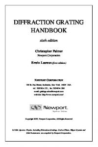
where g and f are certain complex numbers, ξq and ηq are dimensionless Cartesian coordinates of the OV core normalized like Eq. (9); g, f, ξq and ηq generally depend on ζ. The corresponding intensity distribution possesses rectangular symmetry and its constant-level contours are ellipses [27] (see Fig. 3 for examples). Usual characteristics of the OV morphology can be expressed via geometric parameters of these ellipses: angle of orientation θa and the ellipse form-factor (major to minor axes ratio w1/w2) as shown in Fig. 3.
(a)
(b)
θa
Fig. 3. Intensity pattern in the nearest vicinity of the secondary OV cores for the diffracted beam with l = 3, θ = 0.854 rad (σ = 1.5) at the distance ζ = 0.35 after the grating: (a) near the beam axis (axial OV); (b) near the off-axial OV. Ellipses of equal amplitude and the OV morphology parameters are shown. In the numerical analysis, we directly calculate the beam intensity distribution near the expected OV core by means of formula (3) or (12) and afterwards, a contour of constant intensity is
10 determined and fitted by an ellipse whose center, orientation and half-axes are found by using the least square approximation (see Fig. 3). The ellipse center is then identified with the OV core position; other parameters are used for the OV morphology analysis (Sec. 3.2). 3.1. Positions of the OV cores within the beam cross section The high-order OV, expected when |l| > 1 in Eq. (1), can be treated as a “prototype” nonperturbed situation where all the secondary OVs are concentrated on the beam axis (ζ = 0). With further propagation, the single-charged OVs separate and move away from the axis. In agreement with general considerations [1,3–5] and observations of other cases of the high-order OV perturbation [18,19], the total number of the secondary OVs equals to |l|. In accordance with the central symmetry of the transverse beam pattern, mentioned in Sec. 2, in any cross section the OVs are distributed symmetrically with respect to the beam axis. Due to this symmetry, if l is an odd number, one of the single-charged OVs remains on the beam axis. All other OVs (and all the secondary OVs if l is even) are situated in the opposite quadrants of the Gartesian frame. Qualitatively, their positions obey the simple rules formulated primarily for the case of astigmatic transformation of LG modes [18,19] (see Fig. 4 of Ref. [19]). As the beam “contracts” in certain transverse direction, the secondary OVs move as if they are “squeezed out” perpendicularly to the axis of the beam “compression”, simultaneously experiencing certain additional deviation in agreement with handedness of the transverse energy circulation. In all examples of this paper the prototype beam possesses positive l (counter-clockwise energy circulation when viewing against the beam propagation) and is squeezed along the x axis, so the secondary OVs “slip out” along the y axis and, additionally, displace into the 2nd and 4th quadrants of the Cartesian frame (sometimes much farther than in vertical direction, see Fig. 2, bottom row, and Fig. 4). For negative l, the beam patterns would differ by the mirror-like reflection with respect to the vertical axis. This symmetry enables one to consider only the OVs situated at x ≥ 0, which is employed in Figs. 3 – 6. All the formulated regularities of the secondary OVs’ displacements are similar to the analogous properties of the secondary OVs formed under astigmatic transformation of a high-order LG mode [18]. However, the detailed picture of their distribution in the OV beam formed by the “fork” CGH is a bit different. For example, all the secondary OVs, generated after the astigmatic transformation of an LG mode, in every cross section lie on a single straight line intersecting the beam axis [18,19]. To check this property for the situation of this paper, one should note that for |l| ≤ 3 all the OVs lie on a straight line because of clear geometric requirements, including the above mentioned central symmetry. For l = 4 there exists a pair of “inner” secondary OVs and a pair of “outer” ones; Fig. 4 shows those situated in the 4th quadrant. One can see that, in contrast to the data
11 of Refs. [18,19], their cores do not belong to a straight line: there are distinct angles between the solid lines connecting positions of the two OV cores and lines connecting the inner cores with the beam axis, at least for ζ = 0.35 and 0.7. These angles gradually vanish only when ζ → 0 and ζ → ∞.
ηq -0.5
-1.0
0.175 0.35 0.7
-1.5 1.4 -2.5 2.5 0
2.5
5.0
ξq
Fig. 4. Positions of the secondary OVs within the 4th quadrant of the Cartesian frame in the diffracted beam cross section for l = 4, θ = 1.23 rad (70.5°): inner (open circles) and outer (filled circles) OVs of the same cross sections are connected by solid lines, propagation distances in units of ζ are indicated near each filled circle. Another interesting issue related to the secondary OVs is quantitative description of their “moving away” from the axis during the diffracted beam propagation. Besides the general interest, it is important in the light of possible use of such beams for the generation of the OV arrays [18,28– 31]. Corresponding results are presented in Figs. 5 – 7. Fig. 5 and Appendix show that when solving this problem it is convenient to consider an intermediate situation where the output beam deformation described by the coefficient (4) is negligible but decomposition of the expected l-charged OV is already noticeable. In this situation, by using the known expansion 1 3 cos θ ≈ 1 − θ 2 + θ 4 + ... , 2 8
(15)
θ 1 (see Eq. (1)) camn be used for the formation of the OV arrays [28–31]; the existence of the maximum relative separation of the secondary OV cores (Fig. 7) can be a guideline in the search of corresponding transformation arrangement. On the other hand, the analysis presented can serve to more exactly specify the range of validity for approximation cosθ ≈ 1 used in the previous works [11–15], whose important feature is absence of the high-order OV decomposition in the CGH-generated beams. This can be appropriate if the real secondary OV deviation is small compared to the beam transverse size. For example, if the CGH with 16 grooves per millimeter is used (the case of Refs. [12,13]), according to (2), the diffraction angle amounts to θ = 10–2n rad. Due to Eq. (18), this means that for the n-order diffracted beam, separation of secondary OVs roughly equals to n % of the incident beam size, and a noticeably lesser part of the current beam size (in conditions of Refs. [12,13], xq = yq =bξq = bηq ≈ n micrometers). Usually, such a small effect can readily be masked by the noise and/or by the limited resolution of the image analyzing setup, so the secondary OVs visually “combine” into a single high-order OV.
20 Appendix
A.1. Analytical study of the secondary OVs’ separation in case θ 2 and is physically meaningful only at |l| = 3 when it describes the single-charged OV whose position coincides with the “unperturbed” position of the “prototype” high-order OV. In other situations it corresponds to “nonphysical” (|l| – 2)-order OV that does not exist in reality. So, the above reasoning enables us to determine positions of at most three OVs while, in fact, there always exist exactly |l| first-order secondary OVs. “Missing” OVs can be found by the analogous procedure, but higher degrees in expansions (15), (A.1) and (A.2) should be taken into account. For example, if we employ the same approximations but with accuracy of θ4 and again apply conditions (A.10), (A.11), instead of Eq. (A.12) we will have ⎛ i ∂2 1 4 2 ∂4 ⎞ 0 ule (ξ ,η , ζ ) = ⎜ 1 + θ 2ζ − θ ζ u ξ ,η , ζ ) , 2 4 ⎟ le ( 2 ∂ 8 ∂ ξ ξ ⎝ ⎠
(A.18)
the complex amplitude distribution can still be expressed in the form (A.13) but instead of (A.14) and (A.15) we get
i 1 ⎡ ⎤ l −2 P ( Σ ) = ⎢ Σ 4 + θ 2ζ l ( l − 1) Σ 2 − θ 4ζ 2 l ( l − 1)( l − 2 )( l − 3) ⎥ Σ 2 8 ⎣ ⎦
(A.19)
and i 2 1 4 2 ⎡ 4 ⎤ l −2 2 ⎢⎣ Σ (ξ ,η ) + 2 θ ζ l ( l − 1) Σ (ξ ,η ) − 8 θ ζ l ( l − 1)( l − 2 )( l − 3) ⎥⎦ Σ (ξ ,η ) = 0 . (A.20) This equation has already four non-zero solutions 12
⎧ ⎡ 2 ( l − 2 )( l − 3) ⎤ ⎫⎪ ⎪1 ⎥⎬ ξ − ξV = − sgn(l ) (η − ηV ) = ±θ ⎨ ζ l ( l − 1) ⎢1 ± 1 − l ( l − 1) ⎢ ⎥⎪ ⎪⎩ 8 ⎣ ⎦⎭
(A.21)
that describe positions of the secondary OVs when |l| = 4 and 5; for |l| > 5 the “non-perturbed” solution (A.17) is (|l| – 4)-fold and correspond to the nonphysical (|l| – 4)-order OV which can be “decomposed” with allowance for additional terms in expansions (15), (A.1) and (A.2), and so on. A.2. Analytical approximation for arbitrary θ For large θ simplification of the integral (12) is available under condition (19), i.e. in the far field. Then, in the integrand of Eq. (12) the exponent can be transformed as follows: ⎧ i 2 2 ⎫ exp ⎨ ⎡(ξ − ξ a cosθ ) + (η − ηa ) ⎤ ⎬ ⎦⎭ ⎩ 2ζ ⎣ ⎡ i ⎤ ⎡ i ⎤ ≈ exp ⎢ (ξ 2 + η 2 ) ⎥ exp ⎢ − (ξaξ cosθ + ηaη ) ⎥ ⎣ 2ζ ⎦ ⎣ ζ ⎦
23 2 ⎡ i 1 ⎤ × ⎢1 + ξa2 cos2 θ 2 + ηa2 ) − 2 (ξa2 cos2 θ 2 + ηa2 ) + ...⎥ ( 8ζ ⎣ 2ζ ⎦
(A.22)
and function (12) can be represented as ule (ξ ,η , ζ ) =
⎡ i ⎤ 1 ⋅ exp ⎢ (ξ 2 + η 2 ) ⎥ 2π iζ ⎣ 2ζ ⎦
⎡ i ⎛ ∂2 ⎤ ∂2 ⎞ 1 ⎛ ∂4 ∂2 ∂2 ∂4 ⎞ × ⎢1 − ζ ⎜ 2 + 2 ⎟ − ζ 2 ⎜ 4 + 2 2 + + ...⎥ F (ξ cosθ ,η ) 2 4 ⎟ ∂η ⎠ 8 ⎝ ∂ξ ∂ξ ∂η ∂η ⎠ ⎣ 2 ⎝ ∂ξ ⎦
(A.23)
where ⎡ i ⎤ F (ξ ,η ) = ∫ ua (ξ a ,ηa ) eilφ exp ⎢ − (ξ aξ + ηaη ) ⎥ d ξa dηa . ⎣ ζ ⎦ To find explicit representation of this function, note that the far-field form of function (A.4) is ⎡ i ⎤ ule0 (ξ ,η , ζ )ζ →∞ ∝ exp ⎢ (ξ 2 + η 2 ) ⎥ F (ξ ,η ) ; ⎣ 2ζ ⎦ on the other hand, the equivalent expression can be derived from (A.7): ⎡ i ⎤ ule0 (ξ ,η , ζ )ζ →∞ ∝ exp ⎢ (ξ 2 + η 2 ) ⎥ Σ l (ξ ,η ) . ⎣ 2ζ ⎦ As a result, we can accept F (ξ cosθ ,η ) = ⎡⎣Σ (ξ cos θ ,η ) ⎤⎦ . l
(A.24)
Then, after substituting (A.24) into (A.23) and performing the necessary transformations, we obtain the complex amplitude representation in the form ⎡ i ⎤ ule (ξ ,η , ζ ) ∝ exp ⎢ (ξ 2 + η 2 ) ⎥ P ⎡⎣Σ (ξ cosθ ,η ) ⎤⎦ ⎣ 2ζ ⎦
(A.25)
where P(Σ) is given by Eq. (A.19). Expression (A.25) differs from (A.13) only by the first argument of Σ. Positions of the secondary OVs follow from the requirement ule(ξ,η,ζ) = 0 and are determined by equation i 1 2 4 ⎡ 4 ⎤ 2 2 ⎢⎣ Σ (ξ cosθ ,η ) + 2 ζ sin θ l ( l − 1) Σ (ξ cosθ ,η ) − 8 ζ sin θ l ( l − 1)( l − 2 )( l − 3) ⎥⎦ × ⎡⎣Σ (ξ cos θ ,η ) ⎤⎦
l −4
=0.
(A.26)
It appears to be quite similar to (A.20), and its solutions with allowance for (A.8) are similar to (A.21), (A.17):
24
ξ−
ξV
cos θ
= − sgn(l )
(η − ηV ) cos θ
12
⎧ ⎡ 2 ( l − 2 )( l − 3) ⎤ ⎫⎪ ⎪1 ⎥⎬ , = ± tan θ ⎨ ζ l ( l − 1) ⎢1 ± 1 − 8 1 − l l ⎢ ⎥⎪ ( ) ⎣ ⎦⎭ ⎩⎪
ξ−
ξV
cos θ
= η − ηV = 0 .
(A.27)
(A.28)
Note that Eqs. (A.27), (A.28) agree with the fact that in the far field the beam pattern stretches in the x direction proportionally to the squeezing coefficient (4). Like in case of Eq. (A.20), these solutions describe a limited number of separate secondary OVs (at maximum, five), which is connected to the fact that in (A.22) we took only three terms of the exponent expansion (A.2). For |l| > 5, more complete set of the secondary OV positions can be calculated if additional terms in expansion (A.22) are taken into account. A.3. Morphology of the secondary OVs Approximate description of the morphology of the secondary OVs can be obtained directly from the explicit formulas (A.13) and (A.25) for the complex amplitude in close vicinity of the OV cores. Since the exponential prefactor does not affect the intensity distribution, the morphology parameters are fully determined by the polynomial term P(Σ). Obviously, its constant-level contours coincide with those of Σ. This circumstance facilitates the OV morphology analysis in the approximation considered and, simultaneously, restricts its information value by rather trivial results. In case θ