Chord implementation [7]. Note that we ... The conclusion is that erasure coding
is going to matter .... Each node joining the system must download all the data.
High Availability in DHTs: Erasure Coding vs. Replication Rodrigo Rodrigues and Barbara Liskov MIT Abstract
2.1 Replication
High availability in peer-to-peer DHTs requires data redundancy. This paper compares two popular redundancy schemes: replication and erasure coding. Unlike previous comparisons, we take the characteristics of the nodes that comprise the overlay into account, and conclude that in some cases the benefits from coding are limited, and may not be worth its disadvantages.
Replication is the simplest redundancy scheme; here k identical copies of each data object are kept at each instant by system members. The value of k must be set appropriately depending on the desired per object unavailability target, � (i.e., 1 − � has some “number of nines”), and on the average node availability, a. Assuming that node availability is independent and identically distributed (I.I.D.), and assuming we only need one out of the k replicas of the data to be available in order to retrieve it (this would be the case if the data is immutable and therefore a single available copy is sufficient to retrieve the correct object), we compute the following values for �.
1 Introduction Peer-to-peer distributed hash tables (DHTs) propose a logically centralized, physically distributed, hash table abstraction that can be shared simultaneously by many applications [7, 9, 12, 15]. Ensuring that data objects in the DHT have high availability levels when the nodes that are storing them are not themselves 100% available requires some form of data redundancy. Peer-to-peer DHTs have proposed two different redundancy schemes: replication [12, 15] and erasure coding [7, 9]. This paper aims to provide a comprehensive discussion about the advantages of each scheme. While previous comparisons exist [4, 7, 17] they mostly argue that erasure coding is the clear victor, due to huge storage savings for the same availability levels (or conversely, huge availability gains for the same storage levels). Our conclusion is somewhat different: we argue that while gains from coding exist, they are highly dependent on the characteristics of the nodes that comprise the overlay. In fact, the benefits of coding are so limited in some cases that they can easily be outweighed by some disadvantages and the extra complexity of erasure codes. We begin this paper by performing an analytic comparison of replication and coding that clearly delineates the relative gains from using coding vs. replication as a function of the server availability and the desired DHT object availability (Section 2). We present a model [5] that allows us to understand server availability (Section 3). Then we use measured values from three different traces to find out exact values for the parameters of the model (Section 4). This allows us to draw more precise conclusions about the advantages of using coding or replication (Section 5).
2 Coding vs. Replication – Redundancy Levels This section summarizes the two redundancy schemes and presents an analytic comparison that highlights the main advantage of coding: the savings in terms of the required redundancy. Section 5 outlines other positive and negative aspects of the two schemes.
� = P (object o is unavailable) = P (all k replicas of o are unavailable) = P (one replica is unavailable)k = (1 − a)k which upon solving for k yields k=
log � log(1 − a)
(1)
2.2 Erasure Coding With an erasure-coded redundancy scheme, each object is divided into m fragments and recoded into n fragments which are stored separately, where n > m. This means that the effecn . The key property of erasure tive redundancy factor is kc = m codes is that the original object can be reconstructed from any m fragments (where the combined size for the m fragments is approximately equal to the original object size). We now exhibit the equivalent of Equation (1) for the case of erasure coding. (This is a summary of a complete derivation that can be found in [3].) Object availability is given by the probability that at least m out of kc ·m fragments are available: � � k cm X kc m i 1−�= a (1 − a)kc m−i . i i=m Using algebraic simplifications and the normal approximation to the binomial distribution (see [3]), we get the following formula for the erasure coding redundancy factor: q 2 q σ�2 a(1−a) + + 4a σ� a(1−a) m m (2) kc = 2a where σ� is the number of standard deviations in a normal distribution for the required level of availability. E.g., σ� = 3.7 corresponds to four nines of availability.
Replication/Stretch Ratio
3
3 9s 4 9s 5 9s
2.8 2.6 2.4 2.2 2 1.8 1.6 1.4 1.2 0.4
0.5
0.6
0.7
0.8
0.9
1
Server Availability
Figure 1: Ratio between required replication and required expansion factors as a function of the server availability and for three different per-object availability levels. We used m = 7 in equation 2, since this is the value used in the Chord implementation [7].
by the uplink quality (or other factors we are not considering), and the extra DHT availability is in the noise. A question we may ask is why are redundancy savings important? Obviously, they lead to lower disk usage. Also they may improve the speed of writes, since a smaller amount of data has to be uploaded from the writer to the servers, and therefore, if client upload bandwidth limits the write speed, then coding will lead to faster writes. But more important than these two aspects is the savings in the bandwidth required to restore redundancy levels in the presence of changing membership. This importance is due to the fact that bandwidth, and not spare storage, is most likely the limiting factor for the scalability of peer-to-peer storage systems [5].
3 Basic Model
Note that we considered the use of deterministic coding schemes with a constant rate of encoding (e.g., ReedSolomon [13] or IDA [11]). Our analysis does not extend to rateless codes [10], since it is not consensual how to use such codes in a storage environment like a DHT.
This section presents a simple model that allows us to (1) quantify the bandwidth cost for maintaining data redundancy in the presence of membership changes (as a function of the required redundancy), and (2) understand the concept of server availability in a peer-to-peer DHT so we can measure it. The core of the model, described in Sections 3.1 and 3.2, was presented in a previous publication [5], so we will only summarize it.
2.3 Comparing the Redundancy
3.1 Assumptions
The previous discussion highlights the main reason for using coding: the increased redundancy allows the same level of availability to be achieved with much smaller additional storage. The exact gains are depicted in Figure 1. This plots the ratio between the required replication and the required erasure coding expansion factor (i.e., the ratio between equations 1 and 2) for different server availability levels (assuming server availability is I.I.D.) and for three different per-object availability targets: 3, 4, and 5 nines of availability. In this figure we set the number of fragments needed to reconstruct an object to be 7 (i.e., we set m = 7 in Equation 2). This is the value used by Chord [7]. The conclusion is that erasure coding is going to matter more if you store the data in unreliable servers (lower server availability levels) or if you target better guarantees from the system (higher number of nines in object availability). The redundancy gains from using coding range from 1 to 3-fold. The remainder of our discussion assumes a per-object availability target of 4 nines. Targeting higher levels of availability seems exaggerated since other aspects of the system will not keep up with such high availability levels. For instance, a measurement study of MIT’s client access link found that a host at MIT was able to reach the rest of the Internet 99.9% of the time [1]. The same study pointed out that the MIT access link was more reliable than two other links (a DSL line and a 100 Mbits/s link from Cogent). If the client access link only has 3 nines of availability, then making a distinction between, for instance, 5 and 6 nines of of DHT object availability is irrelevant since the end-to-end object availability is dominated
Our model assumes a large, dynamic collection of nodes that cooperatively store data. The data set is partitioned and each subset is assigned to different nodes using a well-known data placement mapping (i.e., a function from the current membership to the set of replicas of each block). This is what happens, for instance, in consistent hashing [8], used by storage systems such as CFS [7]. We make a number of simplifying assumptions. The main simplification comes from the fact that we will only focus on an average-case analysis. When considering the worse-case values for certain parameters, like the rate at which nodes leave the system, the model underestimates the required bandwidth. We assume a fixed redundancy factor and identical pernode space contributions. A previous system [4] dropped these two assumptions and used a variable redundancy factor where many copies are created initially, and, as flaky nodes leave the system, the redundancy levels will drop. This leads to a biased system where the stable nodes donate most of the storage, therefore drastically reducing bandwidth costs. This affects some of our conclusions, and, as future work, we would like to understand how our analysis would change in this new design. We assume a constant rate of joining and leaving and we assume that join and leave events are independent. We also assume a constant steady-state number of nodes.
3.2 Data Maintenance Model We consider a set of N identical hosts that cooperatively provide guaranteed storage over the network. Nodes are added to the set at rate α and leave at rate λ, but the average system size
Membership Interval
Membership Lifetime
Membership Interval
Session Time time
time
Figure 2: Distinction between sessions and lifetimes.
Join
is constant, i.e. α = λ. On average, a node stays a member for T = N/λ (this is a queuing theory result known as Little’s Law [2]). Our data model is that the system reliably stores a total of D bytes of unique data stored with a redundancy factor k, for a total of S = kD bytes of contributed storage. k is either the replication factor or the expansion due to coding and must be set (depending on a desired availability target and on the node availability of the specific deployment) according to equations 1 and 2. Each node joining the system must download all the data that it must serve later, however that subset of data might be mapped to it. The average size of this transfer is S/N , since we assume identical per-node storage contributions. Join events happen every α1 = λ1 time units on average. So the aggregate bandwidth to deal with nodes joining the overlay is λS N , or S/T . When a node leaves the overlay, all the data it housed must be copied over to new nodes; otherwise redundancy would be lost. Thus, each leave event also leads to the transfer of S/N bytes of data. Leaves therefore also require an aggregate bandwidth of λS N , or S/T . In some cases the cost of leaving the system can be avoided: for instance, if the level of redundancy for a given block is sufficiently high, a new node can both join and leave without requiring data movement. We will ignore this optimization and therefore the total 2kD bandwidth usage for data maintenance is 2S T = T , or a per node average of: B/N = 2
kD/N space/node , or BW/node = 2 T lif etime
(3)
3.3 Restoring Redundancy with Coding When coding is used, creating new fragments to cope with nodes holding other fragments leaving the system is not a trivial task. The problem is that with coding schemes like IDA [11], to create a new fragment we must have access to the entire data object. We envision two alternative approaches. The more complicated alternative would be to download enough fragments to reconstruct the object and then create a new fragment. This is very costly since, for each fragment that is lost and needs to be reinstated, some system node needs to download m times the size of the fragment. Thus the amount of data that needs to be transferred is m times higher than the amount of redundancy lost. The alternative is to maintain a full copy of the object at one of the nodes, along with the fragments at the remaining nodes that share the responsibility for the object. In practice, this
Leave
Join
Leave
Figure 3: Membership timeout, τ .
corresponds to increasing the redundancy factors for erasure coding by one unit. Note that the analysis above is still correct when we mix fragments with complete copies, namely the fact that the amount of data that needs to be moved when nodes leave is equal to the amount of data the departing node stored. This is correct because to restore a fragment, the node that keeps a complete copy can create the new fragment and push it to the new owner, and to restore a complete copy the node that will become responsible for that copy can download m fragments with the combined size approximately equal to the size of the object. In the remainder of the paper we will assume that a system using coding keeps the additional complete copy for each object stored in the system.
3.4 Distinguishing Downtime vs. Departure In the model we presented, we refer to joins and leaves as joining the system for the first time or leaving forever, and data movement is triggered only by these events. In other words, we try to make a simple distinction between session times and membership lifetimes (as other authors have noted [3, 14]). This distinction is illustrated in Figure 2: A session time corresponds to the duration of an interval when a node is reachable, whereas a membership lifetime is the time from when the node enters the system for the first time until it leaves the system permanently. This distinction is important since it avoids triggering data movement to restore redundancy due to a temporary disconnection. The side effect of doing this is that nodes will be unavailable for some part of their membership lifetime. We define node availability, a, as the fraction of the time a member of the system is reachable, or in other words, the sum of the node’s session times divided by the node’s membership lifetime.
3.5 Detecting Permanent Departures The problem with this simple model for distinguishing between sessions and membership lifetimes is that it requires future knowledge: applications have no means to distinguish a temporary departure from a permanent leave at the time of a node’s disconnection. To address this problem we introduce a new concept, a membership timeout, τ , that measures how long the system delays its response to failures. In other words, the process of making new hosts responsible for a host’s data does not begin until that host has been out of contact for longer than time τ , as illustrated in Figure 3. There are two main consequences of increasing the membership timeout: First, a higher τ means that member lifetimes
1
Overnet Farsite PlanetLab
Average Availability
Avg Leave Rate (fraction of N/hr)
0.2
0.15
0.1
0.05
0
0.8
Overnet Farsite PlanetLab
0.6
0.4
0.2
0 0
10
20
30
40
50
60
70
80
0
Membership Timeout (hours)
20
30
40
50
60
70
80
Membership Timeout (hours)
Figure 4: Membership dynamics as a function of the membership timeout (τ ).
are longer since transient failures are not considered leaves (and as a consequence the total member count will also increase). Second, the average host availability, a, will decrease if we wait longer before we evict a node from the system. Translating this into our previous model, T and N will now become T (τ ) and N (τ ), and a will now become a(τ ), which implies that k will become k(a(τ ), �) (set accordingly to the equations above). Note that a decreases with τ , whereas T , N , and k increase with τ . By our definition of availability, N (τ ) can be deduced as N (0)/a(τ ). Another consequence is that some joins are not going to trigger data movement, as they will now be re-joins and the node will retain the data it needs to serve after re-joining the system. According to the measurements we will present later, this has a minor impact on data movement when we set long membership timeouts (i.e., if τ is large enough then there will hardly exist any re-joins) so we will ignore this issue. Equation 3 can therefore be rewritten as k(a(τ ), �)D/N (τ ) B/N (τ ) = 2 T (τ )
10
(4)
Note that B/N (τ ) is the average bandwidth used by system members. At any point in time some of these members are not running the application (the unavailable nodes) and these do not contribute to bandwidth usage. Thus we also may want to compute the average bandwidth used by nodes while they are available (i.e., running the application). To do this we replace the left hand side of Equation 4 with a(τ )B/N (0) and compute B/N (0) instead.
4 Measured Dynamics and Availability In this section we present results from measurements of how the membership dynamics and the node availability change as a function of the membership timeout (τ ), and derive the corresponding redundancy requirements and maintenance bandwidth (for both replication and coding). We use numbers from three different traces that correspond to distinct likely deployments of a peer-to-peer storage system: • Peer-to-peer (volunteer-based) – We used the data collected by Bhagwan et al. on their study of the Overnet
Figure 5: Average node availability as a function of the membership timeout (τ ).
file sharing system [3]. This tracked the reachability of 2,400 peers (gathered using a crawl of the system membership) during 7 days by looking up their node IDs every 20 minutes. • Corporate Desktop PCs – We used the data collected by Bolosky et al. [6] on their study of the availability of 51,663 desktop PCs at Microsoft Corporation over the course of 35 days by pinging a fixed set of machines every hour. • Server Infrastructure – This data was collected by Stribling [16] and reflects the results of pinging every pair among 186 hosts of the Planet Lab testbed every 15 minutes. We used the data collected over the course of 70 days between October and December 2003. Here we considered a host to be reachable if at least half of the nodes in the trace could ping it. Our analysis only looks at the average case behavior of the system. Figure 4 shows how increasing the membership timeout τ decreases the dynamics of the system. In this case, the dynamics are expressed as the average fraction of system nodes that leave the system during an hour (in the y axis). Note that by leave we are now referring to having left for over τ units of time (i.e., we are referring to membership dynamics, not session dynamics). As expected, the system membership becomes less dynamic as the membership timeout increases, since some of the session terminations will no longer be considered as membership leaves, namely if the node returns to the system before τ units of time. As mentioned, the second main effect of increasing τ is that the node availability in the system will decrease. This effect is shown in Figure 5. Node availability is, as one would expect, extremely high for PlanetLab (above 97% on average), slightly lower for Farsite (but still above 85% on average), and low for the peer-topeer trace (lower than 50% when τ is greater than 11 hours). Note that we did not plot how N varies with τ but this can be easily deduced from the fact that N (τ ) = N (0)/a(τ ).
Required Redundancy (Stretch)
Required Replication Factor
20
Overnet Farsite PlanetLab
18 16 14 12 10 8 6 4 2 0 0
10
20
30
40
50
60
70
80
Membership Timeout (hours)
Figure 6: Required replication factor for four nines of per-object availability, as a function of the membership timeout (τ ).
4.1 Needed Redundancy and Bandwidth Finally, we measure the bandwidth gains of using erasure coding vs. replication in the three deployments. First, we compute the needed redundancy for the two redundancy schemes as a function of the membership timeout (τ ). To do this we used the availability values of Figure 5 in Equations (1) and (2), and plotted the corresponding redundancy factors, assuming a target average per-object availability of four nines. The results for replication are shown in Figure 6. This shows that Overnet requires the most redundancy, as expected, reaching a replication factor of 20. In the other two deployments replication factors are much lower, on the order of a few units. Note that the replication values in this figure are rounded off to the next integer, since we cannot have a fraction of copies. Figure 7 shows the redundancy requirements (i.e., the expansion factor) for the availability values of Figure 5 (using Equation 2 with m = 7 and four nines of target availability). The redundancy values shown in Figure 7 include the extra copy of the object required to create new fragments as nodes leave the system (as we explained in Section 3.3). As shown in Figure 7, Overnet still requires more redundancy than the other two deployments, but for Overnet coding leads to the most substantial storage savings (for a fixed amount of unique data stored in the system) since it can reduce the redundancy factors by more than half. Finally, we compare the bandwidth usage of the two schemes. For this we use the basic equation for the cost of redundancy maintenance (Equation 3) and apply for membership lifetimes the values implied by the leave rates from Figure 4 (recall the average membership lifetime is the inverse of the average join or leave rate). We will also assume a fixed number of servers (10, 000), and a fixed amount of unique data stored in the system (10T B). We used the replication factors from Figure 6, and for coding the redundancy factors from Figure 7. Figure 8 shows the average bandwidth used for the three different traces and for different values of τ . An interesting effect can be observed in the Farsite trace, where the band-
20
Overnet Farsite PlanetLab
18 16 14 12 10 8 6 4 2 0 0
10
20
30
40
50
60
70
80
Membership Timeout (hours)
Figure 7: Required coding redundancy factor for four nines of per-object availability, as a function of the membership timeout (τ ) as determined by Equation 2, and considering the extra copy required to restore lost fragments.
width has two “steps” (around τ = 14 and τ = 64 hours). These correspond to the people who turn off their machines at night, and during the weekends, respectively. Setting τ to be greater than each of these downtime periods will prevent this downtime from generating a membership change and the corresponding data movement. Figure 9 shows the equivalent of Figure 8 for the case when coding is used instead of replication. The average bandwidth values are now lower due to the smaller redundancy used with coding, especially in the Overnet deployment where we achieve the most substantial redundancy savings.
5 Discussion and Conclusion Several conclusions can be drawn from Figures 8 and 9. For the Overnet trace, coding is a win since server availability is low (we are on the left hand side of Figure 1) but unfortunately the maintenance bandwidth for a scalable and highly available storage system with Overnet-like membership dynamics can be unsustainable for home users (around 100 kbps on average for a modest per-node contribution of a few gigabytes). Therefore, cooperative storage systems should target more stable environments like Farsite or PlanetLab. For the PlanetLab trace, coding is not a win, since server availability is extremely high (corresponding to the right hand side of Figure 1). So the most interesting deployment for using erasure codes is Farsite, where intermediate server availability of 80–90% already presents visible redundancy savings. However, the redundancy savings from using coding instead of full replication come at a price. The main point against the use of coding is that it introduces complexity in the system. Not only there is complexity associated with the encoding and decoding of the blocks, but the entire system design becomes more complex (e.g., the task of redundancy maintenance becomes more complicated as explained in Section 3). As a general principle, we believe that complexity in system design should be avoided unless proven strictly necessary. Therefore system designers should question if the added com-
10000
Overnet Farsite PlanetLab
Maintenance BW (kbps)
Maintenance BW (kbps)
10000
1000
100
10
1
Overnet Farsite PlanetLab
1000
100
10
1 0
10
20
30
40
50
60
70
80
Membership Timeout (hours)
0
10
20
30
40
50
60
70
80
Membership Timeout (hours)
Figure 8: Maintenance bandwidth – Replication. Average bandwidth required for redundancy maintenance as a function of the membership timeout (τ ). This assumes that 10, 000 nodes are cooperatively storing 10T B of unique data, and replication is used for data redundancy.
Figure 9: Maintenance bandwidth – Erasure coding. Average bandwidth required for redundancy maintenance as a function of the membership timeout (τ ). This assumes that 10, 000 nodes are cooperatively storing 10T B of unique data, and coding is used for data redundancy.
plexity is worth the benefits that may be limited depending on the deployment. Another point against the use of erasure codes is the download latency in a environment like the Internet where the internode latency is very heterogeneous. When using replication, the data object can be downloaded from the replica that is closest to the client, whereas with coding the download latency is bounded by the distance to the mth closest replica. This problem was illustrated with simulation results in a previous paper [7]. The task of downloading only a particular subset of the object (a sub-block) is also complicated by coding, where the entire object must be reconstructed. With full replicas sub-blocks can be downloaded trivially. A similar observation is that erasure coding is not adequate for a system design where operations are done at the server side, like keyword searching. A final point is that in our analysis we considered only immutable data. This assumption is particularly important for our distinction between session times and membership lifetimes, because we are assuming that when an unreachable node rejoins the system, its state is still valid. This would not be true if it contained mutable state that had been modified in the meantime. The impact of mutability on the redundancy choices is unclear, since we have to consider how a node determines whether its state is accurate, and what it does if it isn’t. A study of redundancy techniques in the presence of mutability is an area for future work.
[2] D. Bertsekas and R. Gallager. Data Networks. Prentice Hall, 1987. [3] R. Bhagwan, S. Savage, and G. Voelker. Understanding availability. In Proc. IPTPS ’03. [4] R. Bhagwan, K. Tati, Y. Cheng, S. Savage, and G. Voelker. Total recall: System support for automated availability management. In Proc. NSDI ’04. [5] C. Blake and R. Rodrigues. High availability, scalable storage, dynamic peer networks: Pick two. In Proc. 9th HotOS, 2003. [6] W. Bolosky, J. Douceur, D. Ely, and M. Theimer. Feasibility of a serverless distributed file system deployed on an existing set of desktop PCs. In Proc. SIGMETRICS 2000. [7] F. Dabek, J. Li, E. Sit, J. Robertson, F. Kaashoek, and R. Morris. Designing a DHT for low latency and high throughput. In Proc. NSDI ’04. [8] D. Karger, E. Lehman, F. Leighton, M. Levine, D. Lewin, and R. Panigrahy. Consistent hashing and random trees: Distributed caching protocols for relieving hot spots on the world wide web. In Proc. STC’97. [9] J. Kubiatowicz, D. Bindel, Y. Chen, S. Czerwinski, P. Eaton, D. Geels, R. Gummadi, S. Rhea, H. Weatherspoon, W. Weimer, C. Wells, and B. Zhao. Oceanstore: An architecture for globalscale persistent storage. In Proc. ASPLOS 2000. [10] M. Luby. LT codes. In Proceedings of the 43rd Symposium on Foundations of Computer Science (FOCS 2002), Vancouver, Canada, Nov. 2002. [11] M. Rabin. Efficient dispersal of information for security, load balancing, and fault tolerance. J. ACM, 36(2), 1989. [12] S. Ratnasamy, P. Francis, M. Handley, R. Karp, and S. Shenker. A scalable content-addressable network. In Proc. SIGCOMM ’01. [13] S. Reed and G. Solomon. Polynomial codes over certain finite fields. J. SIAM, 8(2):300–304, June 1960. [14] S. Rhea, D. Geels, T. Roscoe, and J. Kubiatowicz. Handling churn in a DHT. In Proc. USENIX’04. [15] A. Rowstron and P. Druschel. Storage management and caching in PAST, a large-scale, persistent peer-to-peer storage utility. In Proc. SOSP’01. [16] J. Stribling. Planetlab - all pairs pings. http://pdos.lcs.mit.edu/ ˜strib/pl app. [17] H. Weatherspoon and J. Kubiatowicz. Erasure coding vs. replication: A quantitative comparison. In Proc. IPTPS ’02.
Acknowledgements We thank Jeremy Stribling, the Farsite team at MSR, and the Total Recall team at UCSD for supplying the data collected in their studies. We thank Mike Walfish, Emil Sit, and the anonymous reviewers for their helpful comments.
References [1] D. Andersen. Improving End-to-End Availability Using Overlay Networks. PhD thesis, MIT, 2005.