High climate velocity and population ... - Wiley Online Library

DOI: 10.1111/ddi.12733

BIODIVERSITY RESEARCH

High climate velocity and population fragmentation may constrain climate-­driven range shift of the key habitat former Fucus vesiculosus Per R. Jonsson1

 | Jonne Kotta2 | Helén C. Andersson3 | Kristjan Herkül2 | 

Elina Virtanen4 | Antonia Nyström Sandman5 | Kerstin Johannesson1 1 Department of Marine Sciences – Tjärnö, University of Gothenburg, Strömstad, Sweden 2

Estonian Marine Institute, University of Tartu, Tallinn, Estonia 3

Swedish Meteorological and Hydrological Institute, Norrköping, Sweden 4

Marine Research Centre, Finnish Environment Institute, Helsinki, Finland 5

AquaBiota Water Research, Stockholm, Sweden Correspondence Per R. Jonsson, Department of Marine Sciences – Tjärnö, University of Gothenburg, Strömstad, Sweden. Email: [email protected] Funding information Vetenskapsrådet; European Union Horizon 2020; Svenska Forskningsrådet Formas; Eesti Teadusagentuur; Seventh Framework Programme; BONUS BIO-C3 project, Grant/ Award Number: 219-2013-2041; Finnish Inventory Programme for the Underwater Marine Environment VELMU; SmartSea project, Grant/Award Number: 292985 Editor: Eric Treml

Abstract Aim: The Baltic Sea forms a unique regional sea with its salinity gradient ranging from marine to nearly freshwater conditions. It is one of the most environmentally impacted brackish seas worldwide, and the low biodiversity makes it particularly sensitive to anthropogenic pressures including climate change. We applied a novel combination of models to predict the fate of one of the dominant foundation species in the Baltic Sea, the bladder wrack Fucus vesiculosus. Location: The Baltic Sea. Methods: We used a species distribution model to predict climate change-­induced displacement of F. vesiculosus and combined these projections with a biophysical model of dispersal and connectivity to explore whether the dispersal rate of locally adapted genotypes may match estimated climate velocities to recolonize the receding salinity gradient. In addition, we used a population dynamic model to assess possible effects of habitat fragmentation. Results: The species distribution model showed that the habitat of F. vesiculosus is expected to dramatically shrink, mainly caused by the predicted reduction of salinity. In addition, the dispersal rate of locally adapted genotypes may not keep pace with estimated climate velocities rendering the recolonization of the receding salinity gradient more difficult. A simplistic model of population dynamics also indicated that the risk of local extinction may increase due to future habitat fragmentation. Main conclusions: Results point to a significant risk of locally adapted genotypes being unable to shift their ranges sufficiently fast considering the restricted dispersal and long generation time. The worst scenario is that F. vesiculosus may disappear from large parts of the Baltic Sea before the end of this century with large effects on the biodiversity and ecosystem functioning. We finally discuss how to reduce this risk through conservation actions, including assisted colonization and assisted evolution. KEYWORDS

Baltic Sea, bladder wrack, climate change, connectivity, dispersal, fragmentation, local adaptation, range shift, salinity, species distribution model

This is an open access article under the terms of the Creative Commons Attribution License, which permits use, distribution and reproduction in any medium, provided the original work is properly cited. © 2018 The Authors. Diversity and Distributions Published by John Wiley & Sons Ltd Diversity and Distributions. 2018;1–14.



wileyonlinelibrary.com/journal/ddi  |  1

|

JONSSON et al.

2      

1 |  I NTRO D U C TI O N

distribution of F. vesiculosus (Vuorinen et al., 2015). A loss of this habitat-­forming species may have far-­reaching consequences and

Owing to the large and densely populated drainage area, the Baltic

lead to changes in biodiversity and functioning of major shallow

Sea is one of the most environmentally impacted seas in the world

ecosystems in the Baltic Sea.

with habitat loss, eutrophication, pollution and overfishing (Diaz &

In this study, we used a species distribution model to predict the

Rosenberg, 2008; Halpern et al., 2008). In addition, recent invasions

current and future distribution of F. vesiculosus under the most plau-

by non-­native species form a strong pressure on the native biota

sible climate and nutrient loading scenarios. In addition, to explore

(Ojaveer & Kotta, 2015). Moreover, the Baltic Sea is one of the fast-

whether locally adapted genotypes of F. vesiculosus (Ardehed et al.,

est warming regions in the world, resulting in dramatic retreat of

2016) may track climate change, we applied a biophysical model to

winter ice cover, rise of surface water temperature and reduction

simulate dispersal, connectivity and ultimately habitat fragmenta-

of salinity (IPCC 2013; Meier, Kjellström, & Graham, 2006; Meier

tion at the receding margin where loss of connectivity may further

et al., 2012a). Low functional diversity of the Baltic marine ecosys-

endanger population persistence (Opdam & Wascher, 2004). The

tem exposes it to fast environmental deterioration and potential loss

modelled rate of dispersal was compared with estimates of climate

of essential ecosystem services due to low resilience capacity (Meier

velocity, calculated as the migration of the isolines of temperature

et al., 2012b; Österblom et al., 2007).

and salinity across the seascape in kilometre per decade (Burrows

Climate-­driven changes in temperature, winter ice cover, salinity

et al., 2011), to assess whether predicted spread of tolerant geno-

and circulation pattern combined with changes in nutrient loading

types is sufficient to match the pace of climate change. Finally, we

affect patterns of habitat availability. Species may track the dis-

discuss potential ecosystem consequences related to shifting pat-

placement in habitat distribution, persist in the altered habitat due

terns in species distribution and connectivity and suggest some

to plasticity or adaptation, or go locally extinct (Chevin, Lande, &

management actions to reduce possible ecosystem impacts.

Mace, 2010; Munday, Warner, Monro, Pandolfi, & Marshall, 2013). Successful range shifts may depend on dispersal capacity of essential genotypes, but changes in distribution pattern, for example increased fragmentation, may also affect the overall metapopulation persistence (Ovaskainen & Hanski, 2003). Clearly, to track environ-

2 | M ATE R I A L S A N D M E TH O DS 2.1 | The study area—the Baltic Sea

mental change, populations must shift their range at least as fast as

The Baltic Sea was formed from a post-­glacial freshwater lake and

does the environment.

is only about 8,000 years old. More than 600 river and stream ba-

Most successful colonizers of the Baltic Sea consist of marine

sins drain into the Baltic Sea that opens to the marine North Sea

and freshwater species with a generally broad salinity tolerance, but

through the shallow Danish straits (Hannerz & Destouni, 2006).

there is growing evidence for many examples of local adaptations

The non-­tidal circulation creates a relatively stable salinity gradient

to the Baltic environment (Berg et al., 2015; Johansson, Pereyra,

through the Baltic Sea from its entrance to the inner parts (Figure

Rafajlovic, & Johannesson, 2017; Momigliano et al., 2017; Pereyra,

S1). The latitudinal extent of the Baltic Sea also produces a strong

Bergström, Kautsky, & Johannesson, 2009; Serrão, Kautsky, &

temperature gradient with a significant development of sea ice in

Brawley, 1996; Sjöqvist, Godhe, Jonsson, Sundqvist, & Kremp, 2015;

the winter–spring season in its northern parts, whereas its southern

Väinölä & Johannesson, 2017). Genetic variation is considered an es-

areas are typically ice-­free. A short geological history, low salinity

sential component for persistence in a changing environment where

and low temperature compared to nearby coastal waters in the east

new genetic combinations or the dispersal of locally adapted geno-

Atlantic make the Baltic Sea a species-­poor ecosystem with key eco-

types may retard the range shift of a species.

system functions often provided by single species (Bonsdorff, 2006;

Bladder wrack (Fucus vesiculosus) is the only canopy-­forming

Bonsdorff & Pearson, 1999).

seaweed on hard bottoms in the Baltic Sea, and it constitutes a key habitat with many associated algae, invertebrate and fish species (Kersen, Kotta, Bučas, Kolesova, & Dekere, 2011; Schagerström,

2.2 | Fucus vesiculosus occurrence

Forslund, Kautsky, Pärnoia, & Kotta, 2014; Wikström & Kautsky,

The distribution data of F. vesiculosus were compiled from several

2007). At present, F. vesiculosus extends into the southern part

sources (Table 1). The HELCOM dataset covered the whole Baltic

of the Gulf of Bothnia, being less common or partly replaced by

Sea with a grid of 10 km × 10 km in which the presence or absence of

its sister species F. radicans further north. Fucus vesiculosus also

F. vesiculosus was assessed. Only records from 1995 to the present

extends into the inner parts of the Gulf of Finland. Locally, re-

(2015) were used. The resulting 10-­km grid served as the input of

duced light availability mostly driven by elevated nutrient loading

current species distribution in the modelling tasks. Recently, a sis-

and phytoplankton production may limit the depth range of F. ve-

ter species to F. vesiculosus was described as F. radicans (Bergström,

siculosus (Torn, Krause-­J ensen, & Martin, 2006). Fucus vesiculosus

Tatarenkov, Johannesson, Jonsson, & Kautsky, 2005), which is en-

thus has rather well-­d efined range margins in the Baltic Sea, and

demic to the Baltic Sea. These two species may occur in the same

predicted climate-­driven changes together with ongoing eutro-

habitat in the northern Baltic Sea (Schagerström et al., 2014) and

phication and habitat fragmentation may all modify the present

they can be difficult to separate based on only morphological traits,

|

      3

JONSSON et al.

TA B L E   1   List of sources for occurrence data of Fucus vesiculosus

Source

References

1. HELCOM Red List dataset

HELCOM (2013)

2. Benthos database of the Estonian Marine Institute, University of Tartu

http://loch.ness.sea. ee/gisservices2/ liikideinfoportaal/

3. Fucus mapping in Schleswig-­Holstein, Germany

Landesamt für Natur und Umwelt des Landes Schleswig-­ Holstein (2008)

4. VELMU database, Finland

http://www. ymparisto.fi/ en-US/VELMU

5. Database of the Swedish national monitoring programme

http://sharkdata.se/

6. Inventory data collected by AquaBiota, Sweden

http://www. aquabiota.se/en/ research-services/ inventories-usingunderwater-video/

and we acknowledge that occurrence data on F. vesiculosus may in-

The RCO-­SCOBI model is a Bryan–Cox–Semtner primitive equa-

clude also F. radicans.

tion circulation model with a free surface and open boundary conditions in the northern Kattegat (Webb, Coward, de Cuevas,

2.3 | Environmental layers from regionalized general circulation model

& Gwilliam, 1997). For the present simulations, RCO-­SCOBI used a horizontal resolution of 3.7 km (2 NM) and with 83 vertical levels with a layer thickness of 3 m. Run-­off changes were calculated

The environmental layers used in the species distribution model

with a hydrological model for the Baltic catchment area (Lind &

(SDM, see below) were produced from simulations of a coupled

Kjellström, 2009). The RCO-­SCOBI model produced the following

physical–biogeochemical model of the Baltic Sea (Meier et al.,

physical and chemical data layers: Secchi depth, salinity, tempera-

2012a) based on one climate change scenario (A1B) and two nutrient

ture, nitrate (NO3) and phosphate (PO 4). Seasonal means for win-

loading scenarios. The A1B climate scenario is a scenario proposed in

ter (December to February), and summer (June to August), were

the Special Report on Emissions Scenarios by the Intergovernmental

calculated for the periods 1978–2007 (current) and 2070–2099

Panel on Climate Change (Nakićenović et al., 2000). The A1 scenario

(future climate).

group describes a future world of very rapid economic growth, a global population that peaks in mid-­century and declines thereafter, and the rapid introduction of new and more efficient technologies.

2.4 | Calculations of climate velocities

The two nutrient emission scenarios included “business-­ as-­ usual

Climate velocity (Burrows et al., 2011) was calculated from the climate

(BAU)” with increased river nutrient concentrations (HELCOM,

scenario layers of projected temperature and salinity as a measure of

2007) and current levels of atmospheric deposition, and a “reference

the speed and direction of change in the Baltic seascape. Climate ve-

scenario (REF)” where nutrient concentrations in rivers and atmos-

locity has been suggested as a useful metric for comparing shifts in

pheric deposition remain at current levels (Eilola, Meier, & Almroth,

species distribution with the rate of climate change (Burrows et al.,

2009).

2011; Pinsky, Worm, Fogarty, Sarmiento, & Levin, 2013). The grids

The Baltic Sea coupled physical–biogeochemical model RCO-­

(3.7 km) of temperature and salinity were first aggregated by calculat-

SCOBI (the Swedish Coastal and Ocean Biogeochemical model

ing the average of 3 × 3 original grid cells. The gradient of scalars E

coupled to the Rossby Centre Ocean circulation model; Eilola

(°C/km or psu/km) between neighbouring grid cells was then calcu-

et al., 2009; Meier, Döscher, & Faxen, 2003) was forced by region-

lated using MATLAB (2016a, MathWorks Inc) for the whole domain

alized atmospheric data from the global climate model ECHAM5

as follows:

(Roeckner et al., 2006) and the A1B emission scenarios for the atmospheric forcing of the three-­dimensional circulation model. The regionalization of the atmospheric forcing was simulated with the coupled atmosphere–ice–ocean model RCAO (the Rossby Centre Atmosphere Ocean model developed at the Swedish Meteorological and Hydrological Institute; Döscher et al., 2002), using an atmospheric horizontal grid of 25 km (Meier et al., 2011).

▿E =

𝜕E 𝜕E + 𝜕x 𝜕𝜆

(1)

where x and y are orthogonal coordinates in space. The climate velocity (km/decade) was then calculated for each grid cell as follows: climate velocity =

1 ⋅ change ▿E

(2)

|

JONSSON et al.

4      

where change is the local change in temperature or salinity per dec-

Random forest (RF) was used as the modelling algorithm. RF is a

ade as calculated from the control period (1978–2007) and future

machine learning method that generates a large number of regres-

layers (2070–2099).

sion trees, each calibrated on a bootstrap sample of the original data (Breiman, 2001). Each node is split using a subset of randomly se-

2.5 | Species distribution model

lected predictors, and the tree is grown to the largest possible extent without pruning. For predicting the value of a new data point, the

The RCO-­ SCOBI model provided environmental layers for the

data are run through each of the trees in the forest and each tree

SDMs. The SDMs incorporated only summer and winter data from

provides a value. The model prediction is then calculated as the aver-

surface (0–3 m) and bottom layers (3–6 m) to optimize the num-

age value over the predictions of all the trees in the forest (Breiman,

ber of candidate models. The climate projection together with

2001). The package “randomforest” (Breiman, Cutler, Liaw, & Wiener,

nutrient emission scenarios resulted in a total of three F. vesicu-

2015) was used to run RF models in the statistical software

losus modelling sets: (1) control period for years 1978–2007, that

(The R Foundation for Statistical Computing 2015). The parameter

is present climate conditions (PRE); (2) future climate conditions

mtry (number of variables randomly sampled as candidates at each

(2070–2099) with nutrient scenario BAU (SCE_BAU); and (3) fu-

split) was set to the square root of the number of variables in the

ture climate conditions (2070–2099) with nutrient scenario REF

model calibration dataset, which is the recommended default value

(SCE_REF).

of mtry in the randomforest package (Liaw & Wiener, 2002), and the

r

3.2.2

In addition to the RCO-­SCOBI data layers, depth and wave expo-

number of trees was set to 1,000 (Liaw & Wiener, 2002). The impor-

sure (simplified wave model) data were also used as modelling input

tance of predictor variables in the PRE model was assessed using

variables. Depth data were acquired from the Baltic Sea Bathymetry

the internal method of the package “randomforest” (mean decrease

Database (Baltic Sea Hydrographic Commission 2013). The model

in accuracy) using 10 permutations (Breiman et al., 2015). Partial de-

of surface wave exposure incorporates shoreline topography, fetch

pendence plots (sensu Friedman, 2001) were produced using par-

and wind data together with empirically derived algorithms to mimic

tialPlot function in “randomforest” to illustrate the dependence of

diffraction (Isæus, 2004). The average values of all RCO-­SCOBI vari-

model predictions on individual covariates. All geographical maps

ables (season × layer × scenario combinations) were added to each

were produced in QGIS or ArcGIS (Esri).

cell of the species distribution data of 10 km. This dataset served as the input for model calibration and prediction. The general concept of species distribution modelling (Elith & Leathwick, 2009) was applied to predict the spatial distribution

2.6 | Biophysical model of dispersal and connectivity

of F. vesiculosus under current and future climate conditions in the

Fucus vesiculosus may disperse in several ways including short-­

Baltic Sea. To investigate which season (summer and winter) and ver-

distance dispersal of gametes and zygotes to occasional long-­

tical layer (surface and bottom) of RCO-­SCOBI data yields the best

distance dispersal of dislodged and rafting buoyant sexually mature

prediction accuracy, candidate models of all season × layer combi-

plants (Rothäusler, Corell, & Jormalainen, 2015; Thiel & Gutow,

nations were calibrated. When building up models, 85% of the input

2005). Also, dispersal on intermediate scales may occur through

data (4,094 data points) were randomly selected and used as model

bed load transport of negatively buoyant plants and in some cases

calibration data, while 15% of the data (722 data points) were re-

vegetative, adventitious branches (Johansson et al., 2017; Pereyra

served for external validation. In the model calibration, the binary

et al., 2013). Genetic studies indicate population structure on

distribution data of F. vesiculosus (presence = 1, absence = 0) were

scales ranging from, in the extreme case 10 m, but more usually

used as the dependent variable and the RCO-­SCOBI layers together

1 km, which suggest relatively short dispersal distances (Muhlin,

with the depth and wave exposure served as independent predic-

Engel, Stessel, Weatherbee, & Brawley, 2008; Tatarenkov, Jonsson,

tors. The probability of occurrence of F. vesiculosus was predicted

Kautsky, & Johannesson, 2007). We estimated the dispersal and

for each of the data points in the validation dataset, and the predic-

connectivity of F. vesiculosus with a biophysical model based on a

tive performance of the candidate models was validated by calcu-

Lagrangian particle-­t racking model driven offline with flow fields

lating the area under the receiver operating curve (AUC) (Fielding

from an ocean circulation model. The stored ocean transport data

& Bell, 1997). The candidate model that produced predictions with

were produced with the NEMO-­ Nordic model (Hordoir, Axell,

the highest AUC value was then used to build final models using

Löptien, Dietze, & Kuznetsov, 2015; Hordoir, Dieterich, Basu,

100% of the input data. All models were calibrated using the present

Dietze, & Meier, 2013), a regional configuration of the NEMO

state (PRE) values of ECHAM5/RCAO variables. The final model pre-

ocean engine (Madec, 2010) covering the Baltic Sea and most of

dictions that covered the whole Baltic Sea were produced for PRE,

the North Sea. It has a horizontal spatial resolution of 3.7 km and

SCE_REF and SCE_BAU datasets. The predicted values of probabil-

84 vertical levels with depth intervals of 3 m at the surface and

ity of occurrence were converted to presence–absence data using

23 m for the deepest layers. Here, tidal harmonics defined the sea

the sensitivity–specificity difference minimizer method (Jiménez-­

surface height (SSH) and velocities, and Levitus climatology de-

Valverde & Lobo, 2007) in the r package “presenceabsence” (Freeman

fined temperature and salinity (Levitus & Boyer, 1994). The model

& Moisen, 2008).

had a free surface, and the atmospheric forcing was the re-­analysis

|

      5

JONSSON et al.

dataset ERA40 (Uppala et al., 2005). Run-­off was based on clima-

simulation. Probabilities were entered into a connectivity matrix

tological data based on a number of different databases for the

where each element represents the probability to disperse from col-

Baltic Sea and the North Sea. Validation of the NEMO-­Nordic

umn i to row j (Jonsson, Nilsson Jacobi, & Moksnes, 2016). Elements

showed that the model is able to correctly represent the SSH, both

along the diagonal represent local retention.

tidally induced and wind-­driven (Hordoir et al., 2015). The Lagrangian trajectory model TRACMASS (De Vries & Döös, 2001) is a particle-­tracking model that calculates transport of particles using stored flow field data. The velocity, temperature and

2.7 | Population model to assess expansion rate and fragmentation

salinity were updated with a regular interval for all grid boxes in

A simplistic metapopulation model for F. vesiculosus was used to

the model domain, in this study every 3 hr, and the trajectory cal-

explore (1) the rate of spread of locally adapted genotypes and (2)

culations were made with a 15-­min time step. Particles simulating

the effect of future fragmentation caused by the predicted changes

zygotes and drifting mature plants were released from all model grid

in habitat distribution and connectivity. The population model con-

cells (3.7 × 3.7 km2) within the HELCOM area that had a mean depth

sidered all sites (habitat grid cells) within the study domain as local

above 10 m or were located adjacent to the land contour. From each

populations connected by dispersal through a connectivity matrix

grid cell, 49 particles were released (a 7 × 7 array) on four occasions

produced by the biophysical model. Every grid cell was given the

between May and August in surface waters (0–2 m), which was re-

same growth rate, and the only mortality occurred for propagules

peated for 8 years (1995–2002), making a total of 20 million parti-

dispersing outside the predicted habitat (from the SDM). The vector

cles. To cover the uncertainty in realized dispersal of F. vesiculosus,

of local population sizes Nt+1 at time t + 1 was simply projected in

particle positions were recorded after 5 and 30 days, representing

time using the connectivity matrix C as:

the range between short-­and long-­distance dispersal. In the final analyses of dispersal and connectivity, only the grid cells contain-

Nt+1 = C ∗ Nt

(3)

ing F. vesiculosus according to the SDM predictions were considered. For each grid cell, the dispersal probability of all other grid cells

For the spread of locally adapted genotypes, an initial population

was calculated from particle positions at the release and end of the

was started at three locations in the Baltic Sea: the western (61.6°N,

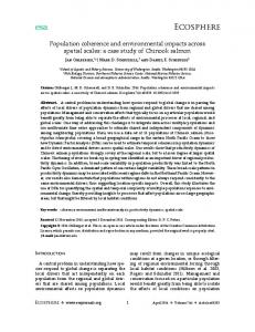
F I G U R E   1   Projected change in sea surface temperature and salinity included in the species distribution model. The change is calculated as the difference between summer means (months June, July and August) for a control period (1978–2007) and a future climate period (2070–2099). (a) Surface temperature and (b) surface salinity

|

JONSSON et al.

6      

17.28°E) and eastern coasts (62.6°N, 21.1°E) of the Gulf of Bothnia

of summer surface sea temperature of about 3–5°C at the end of

and the northern coast (60.4°N, 27.2°E) of the Gulf of Finland. The

this century (Figure 1a). Surface salinity is predicted to decrease

displacements (to the nearest kilometre) of the population front be-

with 1.5–2 psu in most of the Baltic Sea (Figure 1b). The change

tween each of the five successive generations were measured, and

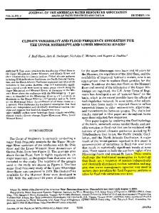
in nutrient loading of nitrogen and phosphorous was evaluated

the front velocity was compared to the calculated climate velocities.

for two scenarios where the business-­a s-­u sual scenario pro-

For the analysis of fragmentation, the population was initiated with

duced higher nutrient concentrations in many areas although

an equal number of individuals in each grid cell predicted as habitat

phosphorous is expected to decrease in the Gulf of Finland

from the SDM for the present distribution and the predicted future for

(Figure 2). With higher nutrient loading resulting in increased

the BAU nutrient scenario. The population was projected for 25 gen-

primary production and plankton biomass, the model predicted

erations, spanning 100 years for F. vesiculosus with an assumed genera-

a general decrease in water transparency with a reduction in

tion time of 4 years (Lüning, 1985). We arbitrarily considered a grid cell

Secchi depth of 1–2 m (Figure 3). However, little change in water

populated by F. vesiculosus over a range of population sizes covering

transparency is expected at the margins of the distribution of

six orders of magnitudes, for example from 1 individual per km2 to 1

F. vesiculosus.

2

individual per 1 m , and as absent below this range. As the model of the spread of locally adapted genotypes did not include mortality or Allee effects, the predicted range expansion is likely an upper bound.

3.2 | Calculated climate velocities From the modelled future change of temperature and salinity,

3 |   R E S U LT S 3.1 | Predicted environment from the RCO-SCOBI scenario model

we calculated fields of climate velocity showing the local rate of change (Figure 4). In particular, the latitudinal velocity of salinity change in the Bothnian Sea and the southern Baltic, and the longitudinal change in the Gulf of Finland, is expected to be rapid with maximum change exceeding 100 km per decade (Figure 4).

The coupled physical–biogeochemical model of the Baltic Sea

The direction of the climate velocity field for salinity is shown in

forced with the climate change scenario A1B predicts an increase

Figure S3.

F I G U R E   2   Projected future difference in nutrient concentrations between a future continuation of the present loads and the business-­ as-­usual scenario. (a) Nitrate and (b) phosphate

|

      7

JONSSON et al.

3.4 | Dispersal of F. vesiculosus The biophysical model showed that a 5-­day drift in surface waters is expected to result in dispersal distances typically between 5 and 15 km along the Baltic Sea coast (Figure 7a). The dispersal direction reflects the general circulation pattern with southward dispersal along the Swedish east coast and northward along the Finnish west coast (Figure 7b).

3.5 | Metapopulation model of fragmentation and genotype range shift In a simplistic metapopulation model, we combined the distribution of F. vesiculosus predicted from SDM with the modelled dispersal in the seascape. The projection of the metapopulation over 25 generations showed that based on the current distribution of F. vesiculosus, the metapopulations are relatively persistent (Figure 8a), although some of the initially inhabited areas were lost, most notably along the eastern Bothnian Sea. The predicted future distribution of F. vesiculosus showed strong effects of fragmentation along the northern distribution boundary in the Bothnian Sea as well as in the Gulf of Finland where suitable habitats, as predicted by SDM, may be difficult to persistently populate (Figure 8b). Such fragmentation may further shift the predicted distribution limits to the south and the F I G U R E   3   Projected future change in water transparency expressed as the Secchi depth, assuming a business-­as-­usual scenario for the nutrient loading

west. The metapopulation model was further used to explore the along-­shore spread of locally adapted genotypes to track their optimal environment under the changing climate conditions. The rate of population expansion from three sites in the Bothnian Sea and the

3.3 | Prediction of future distribution of F. vesiculosus

Gulf of Finland was 35–55 km per decade when assuming dispersal duration of 5 days and around 200 km per decade for regularly occurring long-­distance dispersal lasting for 30 days (Table 2).

The candidate models including different combinations of water layer and seasonal data had very similar predictive performance (AUC values between 0.92 and 0.93). Final predictions of the dis-

4 | D I S CU S S I O N

tribution of F. vesiculosus were produced using bottom water layer (3–6 m) and summer values as this combination yielded marginally

The species distribution model (SDM) based on a regional climate

higher prediction accuracy (AUC = 0.93) compared to the other

model predicts a dramatic 30% reduction of the inhabitable area

combinations.

for the habitat-­forming seaweed F. vesiculosus in the Baltic Sea. The

The predictions of occurrence of F. vesiculosus under future cli-

mechanism behind this range shrinkage is a dramatic southward and

mate and nutrient scenarios are shown in Figure 5. Compared to

westward expansion of low-­salinity water, most notably in the Gulf

the current climate conditions, the nutrient scenarios BAU and REF

of Bothnia and the Gulf of Finland. Although the projected range of

under future climate predicted a reduction of 30% and 33% in the

salinity decline is uncertain, most models in an ensemble simulation

distribution area of F. vesiculosus, respectively. The decrease of dis-

of 16 scenarios showed a decrease in salinity (Meier et al., 2006). In

tribution was most pronounced in the Gulf of Bothnia and the Gulf

addition to the dilution effect, an increasing nutrient load may en-

of Finland. As expected, depth was the most influential predictor

hance plankton primary production leading to reduced water trans-

variable in the RF model used (Figure 6). However, among variables

parency as well as trigger blooms of epiphytic filamentous algae

that were expected to change in future scenarios, the reduced salin-

(Valiela et al., 1997). In either way, F. vesiculosus populations could

ity was the main driver of the change in distribution, while nutrients,

be weakened dramatically. We further show that the loss of suitable

water transparency and other factors had smaller effects (Figure 6).

habitat may result in reduced connectivity leading to lower meta-

Partial dependence plots of predictor variables are shown in the

population persistence and to further fragmentation, especially at

Supporting Information (Figure S2).

the distribution margins where significant losses of local populations

|

8      

JONSSON et al.

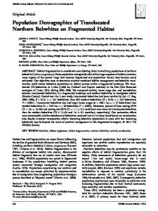
F I G U R E   4   Climate velocity expressed in kilometre per decade. (a) Latitudinal velocity of surface temperature, (b) longitudinal velocity of surface temperature, (c) latitudinal velocity of surface salinity and (d) longitudinal velocity of surface salinity. Climate velocity was calculated for the change between a control period (1978–2007) and a future climate period (2070–2099) for the summer months June, July and August

JONSSON et al.

|

      9

F I G U R E   5   Species distribution model (SDM) of the change in the distribution of Fucus vesiculosus from a control period (1978–2007) to the projected future climate period (2070–2099). (a) Modelled present distribution, (b) modelled distribution assuming a future continuation of present nutrient loading and (c) modelled distribution assuming a business-­as-­usual scenario for the nutrient loading within the metapopulation are expected. This fragmentation effect is likely strong along the Finnish and Estonian coasts. Previous SDM studies have used global climate models in their projections. However, due to the coarse resolution of the global models, they are often not suitable for studies of regional conditions, while higher resolution models can give a more correct representation of air temperature, wind patterns and precipitation. Thus, it is not surprising that the projections of Assis, Serrão, Claro, Perrin, and Pearson (2014) and Leidenberger, De Giovanni, Kulawik, Williams, and Bourlat (2015) came to a different conclusion with a moderate increase in the future distribution of F. vesiculosus within the Baltic Sea. The simulated increase in these studies was mainly driven by an increase in temperature. In contrast, Vuorinen et al. (2015) quan-

F I G U R E   6   Importance of predictor variables in the final random forest model. The x-­axis shows the decrease in accuracy as the increase of mean-­squared error of the model when a variable is permuted

tified the range of low-­salinity area within the Baltic Sea using the same climate scenario model as in the present study. The authors

moon phase (Andersson, Kautsky, & Kalvas, 1994) and the risk of

then compared the shifting salinity conditions with species toler-

beaching (Muhlin et al., 2008). At present, it is not possible to esti-

ances under current environmental conditions and concluded similar

mate the significance of drifting thalli to overall gene flow. Moreover,

range shrinkage under future climate as forecasted in our study.

the oceanographical circulation models (RCO-­SCOBI and NEMO-­

Recent studies have pointed out that predictions of SDMs may

Nordic) cannot accurately simulate currents close to the coast due

both under-­and overestimate future habitat loss if the population

to their relatively coarse spatial resolution. The values in the coastal

consists of locally adapted subpopulations (e.g., Hällfors et al., 2016;

grid cells used in this study are hence likely an overestimate of actual

Oney, Reineking, O’Neill, & Kreyling, 2013). Predictions may be overly

coastal current velocities. In the current paper’s context, the mod-

optimistic if locally adapted genotypes are dispersal-­limited. This

elled dispersal should then be viewed as an upper bound and F. vesic-

may apply to F. vesiculosus where poor dispersal ability with zygotes

ulosus may be even more dispersal-­limited than the model predicted.

or clonal adventitious branches is generally expected (Johansson

Studies of genetic differentiation and morphology suggest that

et al., 2017; Pereyra et al., 2013; Väinölä & Johannesson, 2017).

the population structure of F. vesiculosus in the Baltic Sea may be

Our biophysical model with drift duration of 5 days predicted rela-

very complex with a mix of sexual and asexual recruitment (Ardehed

tively short dispersal distances, generally less than 10 km. Dislodged

et al., 2016). In addition, a closely related species F. radicans has

and drifting adult thalli may travel for longer distances and release

evolved as an endemic species from F. vesiculosus inside the Baltic

gametes far from their native area (Rothäusler et al., 2015), which

Sea (Ardehed et al., 2016; Bergström et al., 2005; Pereyra et al.,

is also indicated for other fucoids (Buonomo et al., 2017). However,

2013). Although genomic information about geographical differ-

dislodged plants may only rarely lead to realized dispersal as spawn-

ences in adaptive loci is lacking, there are indications of trait differ-

ing is often constrained by calm weather (Serrão et al., 1996), the

ences that suggest the presence of locally adapted populations along

|

10      

JONSSON et al.

F I G U R E   7   Dispersal within the Baltic Sea simulated with a biophysical model for propagules drifting in surface water (0–2 m) for a duration of 5 days. (a) Dispersal distance and (b) dispersal direction binned in the four cardinal directions (north: 315°–45°, east: 45°–135°, south: 135°–225°, west: 225°–315°). The data are an average of the years 1995–2002

the Baltic Sea gradient in both these species (Johansson et al., 2017;

direction (Figure 7b), there is a match between directions of climate

Pearson, Kautsky, & Serrão, 2000; Serrão et al., 1996).

velocity of salinity and dispersal along the Swedish coast and within

If locally adapted genotypes will successfully track an advanc-

the Gulf of Finland, but generally a mismatch along the Finnish and

ing or receding optimal environment during a climate change sce-

Estonian coasts. A mismatch for the sessile F. vesiculosus should

nario, the dispersal to and colonization of new areas must occur at

further obstruct a range shift of locally adapted genotypes. The in-

a rate similar to the spatial change of critical environmental factors.

creasing fragmentation of the marginal populations may also reduce

Failing to track a receding critical environment boundary, for exam-

successful dispersal and increase local extinction as predicted by the

ple salinity, may lead to local or even global extinction of unique ge-

metapopulation model (Figure 8). Consequently, there is relatively

netic variants and adaptations. The calculated climate velocities for

high risk that locally adapted populations, evolved to tolerate low

salinity in this study indicate that the dispersal rate is lower or of

salinity in the Bothnian Sea and the Gulf of Finland, may go extinct

the same order as the rate of range shift for F. vesiculosus (Table 2;

under current IPCC climate scenarios. Such inability of adapted gen-

Figure 4). Only if long-­distance dispersal of drifting thalli is an im-

otypes to track the spatial change in the environment may lead to

portant contribution to gene flow, are locally adapted genotypes

an even more severe decline of F. vesiculosus in the future Baltic Sea

expected to outpace the receding boundary of critical salinity. This

than predicted by the SDM as there will be no locally tolerant gen-

also assumes relatively rapid selective sweeps of locally beneficial

otypes when the critical salinity boundary sweeps south-­west. This

alleles (Morjan & Rieseberg, 2004). In addition, García Molinos,

may lead to a reduced tolerance to low salinity at the population

Burrows, and Poloczanska (2017) recently showed that many ongo-

level with F. vesiculosus requiring higher salinity for persistence than

ing range shifts are correlated not only with the climate velocity but

today. This effect may be long-­lasting unless evolution of new locally

also with the directional agreement between climate velocity and

adapted populations is rapid. But the latter is not likely considering

dispersal, especially for species with propagules strongly influenced

the long generation time and the potentially small size of fragmented

by physical water transport. In a qualitative comparison between

populations of F. vesiculosus. There is also a need for more detailed

the direction of decreasing salinity (Figure S3) and mean dispersal

information about the relative contribution of plasticity (Johansson

|

      11

JONSSON et al.

F I G U R E   8   Distribution of Fucus vesiculosus produced by the metapopulation model (eq. 3) where habitat prediction from the species distribution model is combined with the connectivity estimated with a biophysical model. (a) Population density when metapopulation model is based on the present habitat prediction in Figure 6a and (b) population density when metapopulation model is based on the future habitat prediction in Figure 6c. Population density is given in relative units but was modelled as number of thalli per km2

et al., 2017) and local adaptations to salinity tolerance at multiple locations within the present salinity gradient.

& Samuelson, 1999). For some populations, as in the northern Baltic Sea with high rates of asexual reproduction (Ardehed et al., 2016),

A dramatic decline of F. vesiculosus due to reduced salinity will

it may be possible to translocate clonal copies using adventitious

likely be accompanied by a severe structural and functional regime

branches of tolerant clones (Johannesson, Smolarz, Grahn, & André,

shift of the coastal ecosystem including a dramatic loss of biodiver-

2011). Ultimately, even evolution could be assisted where genotypes

sity in the Baltic Sea (Kotta, Möller, Orav-­Kotta, & Pärnoia, 2014;

are selected that are more tolerant to a rapidly changing environ-

Vuorinen et al., 2015). Much of brackish and marine vegetation will

ment (van Oppen, Oliver, Putnam, & Gates, 2015). Artificial selection

be replaced by freshwater higher plants (Kotta et al., 2014). However,

may be a challenge for F. vesiculosus considering its long generation

none of the freshwater habitat-­building species can replace F. vesic-

time of over 4 years.

ulosus on rocky bottoms. Consequently, such habitats will likely lose much of their extant vegetation, become less complex and species-­ poor and be deprived of critical ecosystem services such as nutrient uptake, food source, refuge for juvenile fish and loss of aesthetic values for recreational activities. It is possible that if dispersal and colonization are sufficiently fast, the sister species F. radicans may replace F. vesiculosus in areas where salinity decreases over time,

TA B L E   2   Rate of population expansion from three selected locations in the Gulf of Bothnia and the Gulf of Finland Location West Bothnian Bay

which could maintain canopies on rocky substrates. Further studies are here needed.

East Bothnian Bay

Conservation actions may mitigate the effect of low dispersal of locally adapted populations. Assisted dispersal and colonization through translocation of individuals of Fucus or zygotes is one option (Hiddink, Ben Rais Lasram, Cantrill, & Davies, 2012; Thomas, 2011). It may be even possible to produce zygotes or seedlings through assisted spawning and fertilization (Serrão, Brawley, Hedman, Kautsky,

Gulf of Finland

Drift duration (days)

Expansion rate (km/decade)

5

36

30

226

5

41

30

37

5

57

30

250

Rates are shown for two dispersal strategies with drift duration of either 5 or 30 days in surface waters (0–2 m) as a mean for the period May–August.

|

JONSSON et al.

12      

AC K N OW L E D G E M E N T S This work was carried out within the Linnaeus Centre for Marine Evolutionary Biology at the University of Gothenburg (www.cemeb. science.gu.se/). PRJ was supported by the Swedish Research Council, by the EU FP Horizon 2020 within the MARFOR project and through the projects BAMBI and BIO-­C3, which received funding from BONUS, the joint Baltic Sea research and development programme (EU FP7 Art 185 and FORMAS). JK and KH were also supported by institutional research funding IUT02-­20 of the Estonian Research Council. HCA was funded by the BONUS BIO-­C3 project (EU FP7 Art 185 and FORMAS Grant No. 219-­2013-­2041). E.V. acknowledges the SmartSea project (Grant no. 292985), funded by the Strategic Research Council of the Academy of Finland, and the Finnish Inventory Programme for the Underwater Marine Environment VELMU, funded by the Ministry of the Environment Finally, we thank two anonymous reviewers for constructive comments on the manuscript.

DATA ACC E S S I B I L I T Y If required, modelled data on present and future distributions of F. vesiculosus may be archived at Dryad Digital Repository with a 1-­ year embargo.

ORCID Per R. Jonsson 

http://orcid.org/0000-0002-1793-5473

REFERENCES Andersson, S., Kautsky, L., & Kalvas, A. (1994). Circadian and lunar gamete release in Fucus vesiculosus in the atidal Baltic Sea. Marine Ecology Progress Series, 110, 195–201. https://doi.org/10.3354/meps110195 Ardehed, A., Johansson, D., Sundqvist, L., Schagerström, E., Zagrodzka, Z., Kovaltchouk, N., … Johannesson, K. (2016). Divergence within and among Seaweed Siblings (Fucus vesiculosus and F. radicans) in the Baltic Sea. PLoS ONE, 11, e0161266. https://doi.org/10.1371/journal.pone.0161266 Assis, J., Serrão, E., Claro, B., Perrin, C., & Pearson, G. A. (2014). Climate-­driven range shifts explain the distribution of extant gene pools and predict future loss of unique lineages in a marine brown alga. Molecular Ecology, 23, 2797–2810. https://doi.org/10.1111/ mec.12772 Baltic Sea Hydrographic Commission. (2013). Baltic Sea Bathymetry Database, version 0.9.3. Available at: (accessed April 24, 2017) Berg, P. R., Jentoft, S., Star, B., Ring, K. H., Knutsen, H., Lien, S., … Andre ,́ C. (2015). Adaptation to low salinity promotes genomic divergence in Atlantic cod (Gadus morhua L.). Genome Biology and Evolution, 7, 1644–1663. https://doi.org/10.1093/gbe/evv093 Bergström, L., Tatarenkov, A., Johannesson, K., Jonsson, R. B., & Kautsky, L. (2005). Genetic and morphological identification of Fucus radicans sp Nov (Fucales, Phaeophyceae) in the brackish Baltic Sea. Journal of Phycology, 41, 1025–1038. https://doi. org/10.1111/j.1529-8817.2005.00125.x Bonsdorff, E. (2006). Zoobenthic diversity-­gradients in the Baltic Sea: Continuous post-­glacial succession in a stressed ecosystem. Journal of Experimental Marine Biology and Ecology, 330, 383–391. https:// doi.org/10.1016/j.jembe.2005.12.041

Bonsdorff, E., & Pearson, T. H. (1999). Variation in the sublittoral macrozoobenthos of the Baltic Sea along environmental gradients: A functional-­group approach. Australian Journal of Ecology, 24, 312– 326. https://doi.org/10.1046/j.1442-9993.1999.00986.x Breiman, L. (2001). Random forests. Machine Learning, 45, 5–32. https:// doi.org/10.1023/A:1010933404324 Breiman, L., Cutler, A., Liaw, A., & Wiener, M. (2015). randomForest: Breiman and Cutler’s random forests for classification and regression. R package version 4.6-12. Available at: http://cran.r-project.org/web/ packages/randomForest/ (accessed April 24, 2017) Buonomo, R., Assis, J., Fernandes, F., Engelen, A. H., Airoldi, L., & Serrão, E. (2017). Habitat continuity and stepping-­stone oceanographic distances explain population genetic connectivity of the brown alga Cystoseira amentacea. Molecular Ecology, 26, 766–780. https://doi. org/10.1111/mec.13960 Burrows, M. T., Schoeman, D. S., Buckley, L. B., Moore, P., Poloczanska, E. S., Brander, K. M., … Bruno, J. F. (2011). The pace of shifting climate in marine and terrestrial ecosystems. Science, 334, 652–655. https:// doi.org/10.1126/science.1210288 Chevin, L. M., Lande, R., & Mace, G. M. (2010). Adaptation, plasticity, and extinction in a changing environment: Towards a predictive theory. PLoS Biology, 8, e1000357. De Vries, P., & Döös, K. (2001). Calculating Lagrangian trajectories using time-­dependent velocity fields. Journal of the Atmospheric Sciences, 18, 1092–1101. Diaz, R. J., & Rosenberg, R. (2008). Spreading dead zones and consequences for marine ecosystems. Science, 321, 926–929. https://doi. org/10.1126/science.1156401 Döscher, R., Willén, U., Jones, C., Rutgersson, A., Meier, H. E. M., Hansson, U., & Graham, L. P. (2002). The development of the regional coupled ocean-­atmosphere model RCAO. Boreal Environmental Research, 7, 183–192. Eilola, K., Meier, H. E. M., & Almroth, E. (2009). On the dynamics of oxygen, phosphorous and cyanobacteria in the Baltic Sea: A model study. Journal of Marine Systems, 75, 163–184. https://doi.org/10.1016/j. jmarsys.2008.08.009 Elith, J., & Leathwick, J. R. (2009). Species distribution models: Ecological explanation and prediction across space and time. Annual Review of Ecology Evolution and Systematics, 40, 677–697. https://doi. org/10.1146/annurev.ecolsys.110308.120159 Fielding, A. H., & Bell, J. F. (1997). A review of methods for the assessment of prediction errors in conservation presence/absence models. Environmental Conservation, 24, 38–49. https://doi.org/10.1017/ S0376892997000088 Freeman, E. A., & Moisen, G. (2008). PresenceAbsence: An R package for presence-­absence model analysis. Journal of Statistical Software, 23, 1–31. Friedman, J. H. (2001). Greedy function approximation: A gradient boosting machine. Annals of Statistics, 29, 1189–1232. https://doi. org/10.1214/aos/1013203451 García Molinos, J., Burrows, M. T., & Poloczanska, E. S. (2017). Ocean currents modify the coupling between climate change and biogeographical shifts. Scientific Reports, 7, 1332. https://doi.org/10.1038/ s41598-017-01309-y Hällfors, M. H., Liao, J., Dzurisin, J., Grundel, R., Hyvärinen, M., Towle, K., … Hellmann, J. J. (2016). Addressing potential local adaptation in species distribution models: Implications for conservation under climate change. Ecological Applications, 26, 1154–1169. https://doi. org/10.1890/15-0926 Halpern, B. S., Walbridge, S., Selkoe, K. A., Kappel, C. V., Micheli, F., D’Agrosa, C., … Watson, R. (2008). A global map of human impact on marine ecosystems. Science, 319, 948–952. https://doi.org/10.1126/ science.1149345 Hannerz, F., & Destouni, G. (2006). Characterization of the Baltic Sea drainage basin and its unmonitored catchments. Ambio, 35, 214–219. https://doi.org/10.1579/05-A-022R.1

JONSSON et al.

HELCOM. (2007). Climate change in the Baltic Sea area. HELCOM Thematic Assessment in 2007. In Baltic Sea Environment Proceedings HELCOM. (2013). Fucus vesiculosus species information datasheet. In HELCOM Red List Macrophyte Expert Group Hiddink, J. G., Ben Rais Lasram, F., Cantrill, J., & Davies, A. J. (2012). Keeping pace with climate change: What can we learn from the spread of Lessepsian migrants? Global Change Biology, 18, 2161– 2172. https://doi.org/10.1111/j.1365-2486.2012.02698.x Hordoir, R., Axell, L., Löptien, U., Dietze, H., & Kuznetsov, I. (2015). Influence of sea level rise on the dynamics of salt inflows in the Baltic Sea. Journal of Geophysical Research -­Oceans, 120, 6653–6668. https://doi.org/10.1002/2014JC010642 Hordoir, R., Dieterich, C., Basu, B., Dietze, H., & Meier, H. E. M. (2013). Freshwater outflow of the Baltic Sea and transport in the Norwegian current: A statistical correlation analysis based on a numerical experiment. Continental Shelf Research, 64, 1–9. https://doi.org/10.1016/j. csr.2013.05.006 IPCC. (2013). Climate change 2013: The physical science basis. Contribution of Working Group I to the Fifth Assessment Report of the Intergovernmental Panel on Climate Change. Cambridge: Cambridge University Press. Isæus, M. (2004). Factors structuring Fucus communities at open and complex coastlines in the Baltic Sea. PhD thesis, Stockholm. Jiménez-Valverde, A., & Lobo, J. M. (2007). Threshold criteria for conversion of probability of species presence to either–or presence– absence. Acta Oecologica, 31, 361–369. https://doi.org/10.1016/j. actao.2007.02.001 Johannesson, K., Smolarz, K., Grahn, M., & André, C. (2011). The future of Baltic Sea populations: Local extinction or evolutionary rescue? Ambio, 40, 179–190. https://doi.org/10.1007/ s13280-010-0129-x Johansson, D., Pereyra, R. T., Rafajlovic, M., & Johannesson, K. (2017). Reciprocal transplants support a plasticity-­first scenario during colonisation of a large hyposaline basin by a marine macro alga. BMC Ecology, 5, 17. Jonsson, P. R., Nilsson Jacobi, M., & Moksnes, P. O. (2016). How to select networks of marine protected areas for multiple species with different dispersal strategies. Diversity and Distributions, 22, 161–173. https://doi.org/10.1111/ddi.12394 Kersen, P., Kotta, J., Bučas, M., Kolesova, N., & Dekere, Z. (2011). Epiphytes and associated fauna on the brown alga Fucus vesiculosus in the Baltic and the North Seas in relation to different abiotic and biotic variables. Marine Ecology, 32, 87–95. https://doi. org/10.1111/j.1439-0485.2010.00418.x Kotta, J., Möller, T., Orav-Kotta, H., & Pärnoia, M. (2014). Realized niche width of a brackish water submerged aquatic vegetation under current environmental conditions and projected influences of climate change. Marine Environmental Research, 102, 88–101. https://doi. org/10.1016/j.marenvres.2014.05.002 Landesamt für Natur und Umwelt des Landes Schleswig-Holstein. (2008). Kartierung mariner Pflanzenbestände im Flachwasser der Ostseeküste – Schwerpunkt Fucus und Zostera. Außenküste der Schleswig-Holsteinischen Ostsee und Schlei. Kronshagen: Pirwitz Druck & Design. Leidenberger, S., De Giovanni, R., Kulawik, R., Williams, A. R., & Bourlat, S. J. (2015). Mapping present and future potential distribution patterns for a meso-­grazer guild in the Baltic Sea. Journal of Biogeography, 42, 241–254. https://doi.org/10.1111/jbi.12395 Levitus, S., & Boyer, T. P. (1994). World ocean atlas, vol. 5, salinity. NOAA atlas. Liaw, A., & Wiener, M. (2002). Classification and regression by randomForest. R News, 2, 18–22. Lind, P., & Kjellström, E. (2007). Water budget in the Baltic Sea drainage basin: Evaluation of simulated fluxes in a regional climate model. Boreal Environment Research, 14, 56–67. Lüning, K. (1985). Meeresbotanik. Verbreitung, Ökophysiologie und Nutzung der marinen Makroalgen. Thieme Verlag: Stuttgart.

|

      13

Madec, G. (2010). Nemo ocean engine, version 3.3, Tech. rep., IPSL. MATLAB Release (2016a). The MathWorks, Inc., Natick, Massachusetts, United States. Meier, H. E. M., Andersson, H. C., Arheimer, B., Blenckner, T., Chubarenko, B., Donnelly, C., … Zorita, E. (2012b). Comparing reconstructed past variations and future projections of the Baltic Sea ecosystem-­first results from multi-­model ensemble simulations. Environmental Research Letters, 7, 034005. https://doi.org/10.1088/1748-9326/7/3/034005 Meier, H. E. M., Döscher, R., & Faxen, T. (2003). A multiprocessor coupled ice-­ocean model for the Baltic Sea: Application to salt inflow. Journal of Geophysical Research -­Oceans, 108, 3273. https://doi. org/10.1029/2000JC000521 Meier, H. E. M., Höglund, A., Döscher, R., Andersson, H., Löptien, U., & Kjellström, E. (2011). Quality assessment of atmospheric surface fields over the Baltic Sea from an ensemble of regional climate model simulations with respect to ocean dynamics. Oceanologia, 53, 193– 227. https://doi.org/10.5697/oc.53-1-TI.193 Meier, H. E. M., Hordoir, R., Andersson, H. C., Dieterich, C., Eilola, K., Gustafsson, B. G., … Schimanke, S. (2012a). Modeling the combined impact of changing climate and changing nutrient loads on the Baltic Sea environment in an ensemble of transient simulations for 1961– 2099. Climate Dynamics, 39, 2421–2441. https://doi.org/10.1007/ s00382-012-1339-7 Meier, H. E. M., Kjellström, E., & Graham, P. (2006). Estimating uncertainties of projected Baltic Sea salinity in the late 21st century. Geophysical Research Letters, 33, L15705. https://doi. org/10.1029/2006GL026488 Momigliano, P., Jokinen, H., Fraimout, A., Florin, A.-B., Norkko, A., & Merilä, J. (2017). Extraordinarily rapid speciation in a marine fish. Proceedings of the National Academy of Sciences of the United States of America, 114, 6074–6079. https://doi.org/10.1073/ pnas.1615109114 Morjan, C. L., & Rieseberg, L. H. (2004). How species evolve collectively: Implications of gene flow and selection for the spread of advantageous alleles. Molecular Ecology, 13, 1341–1356. https://doi. org/10.1111/j.1365-294X.2004.02164.x Muhlin, J. F., Engel, C. R., Stessel, R., Weatherbee, R. A., & Brawley, S. H. (2008). The influence of coastal topography, circulation patterns, and rafting in structuring populations of an intertidal alga. Molecular Ecology, 17, 1198–1210. https://doi.org/10.1111/j.1365-294X.2007.03624.x Munday, P. L., Warner, R. R., Monro, K., Pandolfi, J. M., & Marshall, D. J. (2013). Predicting evolutionary responses to climate change in the sea. Ecology Letters, 16, 1488–1500. https://doi.org/10.1111/ ele.12185 Nakićenović, N., Alcamo, J., Davis, G., DeVries, B., Fenhann, J., Gaffin, S., … Dadi, Z. (2000). Special report on emissions scenarios: A special report of Working Group III of the Intergovernmental Panel on Climate Change. Cambridge: Cambridge University Press. Ojaveer, H., & Kotta, J. (2015). Ecosystem impacts of the widespread non-­indigenous species in the Baltic Sea: Literature survey evidences major limitations in knowledge. Hydrobiologia, 750, 171–185. https:// doi.org/10.1007/s10750-014-2080-5 Oney, B., Reineking, B., O’Neill, G., & Kreyling, J. (2013). Intraspecific variation buffers projected climate change impacts on Pinus contorta. Ecology and Evolution, 3, 437–449. https://doi.org/10.1002/ece3.426 Opdam, P., & Wascher, D. (2004). Climate change meets habitat fragmentation: Linking landscape and biogeographical scale levels in research and conservation. Biological Conservation, 117, 285–297. https://doi. org/10.1016/j.biocon.2003.12.008 van Oppen, M. J. H., Oliver, J. K., Putnam, H. M., & Gates, R. D. (2015). Building coral reef resilience through assisted evolution. Proceedings of the National Academy of Sciences of the United States of America, 112, 2307–2313. https://doi.org/10.1073/pnas.1422301112 Österblom, H., Hansson, S., Larsson, U., Hjerne, O., Wulff, F., Elmgren, R., & Folke, C. (2007). Human-­induced trophic cascades and ecological

|

JONSSON et al.

14      

regime shifts in the Baltic Sea. Ecosystems, 10, 877–889. https://doi. org/10.1007/s10021-007-9069-0 Ovaskainen, O., & Hanski, I. (2003). How much does an individual habitat fragment contribute to metapopulation dynamics and persistence? Theoretical Population Biology, 64, 481–495. https://doi.org/10.1016/ S0040-5809(03)00102-3 Pearson, G., Kautsky, L., & Serrão, E. (2000). Recent evolution in Baltic Fucus vesiculosus: Reduced tolerance to emersion stresses compared to intertidal (North Sea) populations. Marine Ecology Progress Series, 202, 67–79. https://doi.org/10.3354/meps202067 Pereyra, R. T., Bergström, L., Kautsky, L., & Johannesson, K. (2009). Rapid speciation in a newly opened postglacial marine environment, the Baltic Sea. BMC Evolutionary Biology, 9, 70. https://doi. org/10.1186/1471-2148-9-70 Pereyra, R. T., Huenchuñir, C., Johansson, D., Forslund, H., Kautsky, L., Jonsson, P. R., & Johannesson, K. (2013). Parallel speciation or long-­distance dispersal? Lessons from seaweeds (Fucus) in the Baltic Sea. Journal of Evolutionary Biology, 26, 1727–1737. https://doi. org/10.1111/jeb.12170 Pinsky, M. L., Worm, B., Fogarty, M. J., Sarmiento, J. L., & Levin, S. A. (2013). Marine taxa track local climate velocities. Science, 341, 1239– 1242. https://doi.org/10.1126/science.1239352 Roeckner, E., Brokopf, R., Esch, M., Giorgetta, M., Hagemann, S., Kornblueh, L., … Schulzweida, U. (2006). Sensitivity of simulated climate to horizontal and vertical resolution in the ECHAM5 atmosphere model. Journal of Climate, 19, 3771–3791. https://doi. org/10.1175/JCLI3824.1 Rothäusler, E., Corell, H., & Jormalainen, V. (2015). Abundance and dispersal trajectories of floating Fucus vesiculosus in the Northern Baltic Sea. Limnology and Oceanography, 60, 2173–2184. https://doi. org/10.1002/lno.10195 Schagerström, E., Forslund, H., Kautsky, L., Pärnoia, M., & Kotta, J. (2014). Does thalli complexity and biomass affect the associated flora and fauna of two co-­occurring Fucus species in the Baltic Sea? Estuarine, Coastal and Shelf Science, 149, 187–193. https://doi.org/10.1016/j. ecss.2014.08.022 Serrão, E., Brawley, S. H., Hedman, J., Kautsky, L., & Samuelson, G. (1999). Reproductive success of Fucus vesiculosus (Phaeophyceae) in the Baltic Sea. Journal of Phycology, 35, 254–269. https://doi. org/10.1046/j.1529-8817.1999.3520254.x Serrão, E., Kautsky, L., & Brawley, S. H. (1996). Distributional success of the marine seaweed Fucus vesiculosus L. in the brackish Baltic Sea correlates with osmotic capabilities of Baltic gametes. Oecologia, 107, 1–12. https://doi.org/10.1007/BF00582229 Sjöqvist, C., Godhe, A., Jonsson, P. R., Sundqvist, L., & Kremp, A. (2015). Local adaptation and oceanographic connectivity patterns explain genetic differentiation of a marine diatom across the North Sea-­Baltic Sea salinity gradient. Molecular Ecology, 24, 2871–2885. https://doi.org/10.1111/mec.13208 Tatarenkov, A., Jonsson, R. B., Kautsky, L., & Johannesson, K. (2007). Genetic structure in populations of Fucus vesiculosus (Phaeophyceae) over spatial scales from 10 m to 800 km. Journal of Phycology, 43, 675–685. https://doi.org/10.1111/j.1529-8817.2007.00369.x The R Foundation for Statistical Computing. (2015). R version 3.2.2. Available at: http://www.r-project.org/ (accessed April 24, 2017). Thiel, M., & Gutow, L. (2005). The ecology of rafting in the marine environment. I. The floating substrata. Oceanography and Marine Biology, 42, 181–264. Thomas, C. D. (2011). Translocation of species, climate change, and the end of trying to recreate past ecological communities. Trends in Ecology and Evolution, 26, 216–221. https://doi.org/10.1016/j. tree.2011.02.006 Torn, K., Krause-Jensen, D., & Martin, G. (2006). Present and past depth distribution of bladderwrack (Fucus vesiculosus) in the

Baltic Sea. Aquatic Botany, 84, 53–62. https://doi.org/10.1016/j. aquabot.2005.07.011 Uppala, S. M., Källberg, P. W., Simmons, A. J., Andrae, U., Da Costa Bechtold, V., Fiorino, M., … Woollen, J. (2005). The ERA-­ 4 0 re-­ analysis. Quarterly Journal of the Royal Meteorological Society, 131, 2961–3012. https://doi.org/10.1256/qj.04.176 Väinölä, R., & Johannesson, K. (2017). Genetic diversity and evolution. In P. Snoeijs-Leijonmalm, H. Schubert, & T. Radziejewska (Eds.), Biological oceanography of the Baltic Sea (pp. 233–253). Dordrecht: Springer Science+Business Media. Valiela, I., McClelland, J., Hauxwell, J., Behr, P. J., Hersh, D., & Foreman, K. (1997). Macroalgal blooms in shallow estuaries: Controls and ecophysiological and ecosystem consequences. Limnology and Oceanography, 42, 1105–1118. https://doi.org/10.4319/ lo.1997.42.5_part_2.1105 Vuorinen, I., Hänninen, J., Rajasilta, M., Laine, P., Eklund, J., MontesinoPouzols, F., … Dippner, J. W. (2015). Scenario simulations of future salinity and ecological consequences in the Baltic Sea and adjacent North Sea areas–implications for environmental monitoring. Ecological Indicators, 50, 196–205. https://doi.org/10.1016/j.ecolind.2014.10.019 Webb, D. J., Coward, A. C., de Cuevas, B. E., & Gwilliam, C. S. (1997). A multiprocessor ocean circulation model using message passing. Journal of Atmospheric and Oceanic Technology, 14, 175–183. https://doi.org/10. 1175/1520-0426(1997)0142.0.CO;2 Wikström, S. A., & Kautsky, L. (2007). Structure and diversity of invertebrate communities in the presence and absence of canopy-­forming Fucus vesiculosus in the Baltic Sea. Estuarine, Coastal and Shelf Science, 72, 168–176. https://doi.org/10.1016/j.ecss.2006.10.009

BIOSKETCH Per R. Jonsson is interested in how dispersal of marine organisms affects demography, evolution and strategies for management and conservation. Our research group covers multiple disciplines from several institutions with expertise in ocean circulation, climate change, population dynamics, ecophysiology, phylogeography and evolutionary biology to understand how biodiversity and ecosystem functions may adjust to global changes. Author contributions: PRJ and JK conceived the ideas and designed the study; HCA provided modelled ocean circulation and climate projections; KJ contributed to the discussion of population genetics; KH, EV and ANS provided occurrence data; PRJ and JK led the writing of the manuscript. All authors contributed critically to the draft and gave the final approval for publication.

SUPPORTING INFORMATION Additional Supporting Information may be found online in the ­supporting information tab for this article. 

How to cite this article: Jonsson PR, Kotta J, Andersson HC, et al. High climate velocity and population fragmentation may constrain climate-­driven range shift of the key habitat former Fucus vesiculosus. Divers Distrib. 2018;00:1–14. https://doi.org/10.1111/ddi.12733