Apr 25, 2017 - Antonelli, Joseph, Cefalu, Matthew, Palmer, Nathan, & Agniel, Denis. ... Patel, Chirag J, Cullen, Mark R, Ioannidis, John PA, & Butte, Atul J.
High dimensional confounding adjustment using continuous spike and slab priors Joseph Antonelli, Giovanni Parmigiani, Francesca Dominici
arXiv:1704.07532v1 [stat.ME] 25 Apr 2017
Abstract In observational studies, estimation of a causal effect of a treatment on an outcome relies on proper adjustment for confounding. If the number of the potential confounders (p) is larger than the number of observations (n), then direct control for all these potential confounders is infeasible. Existing approaches for dimension reduction and penalization are for the most part aimed at predicting the outcome, and are not suited for estimation of causal effects. We propose continuous spike and slab priors on the regression coefficients βj corresponding to the potential confounders Xj when p ≥ n. If Xj is associated with the treatment, then we increase the prior probability that βj is included in the slab component of the prior. This reduces the degree of shrinkage of βj towards zero. By using theoretical considerations and a simulation study we compare our proposed approach to alternatives and show its ability to adjust for confounding across a range of data generating mechanisms. Finally, we estimate the causal effects of persistent pesticide exposure on triglyceride levels, which highlights the key important features of our approach: 1) ability to identify the true confounders, and 2) ability to exclude strong instrumental variables, therefore minimizing bias and improving efficiency of effect estimates. High-dimensional data; Causal inference; Bayesian variable selection; Shrinkage priors
1
Introduction
In observational studies, we are often interested in estimating the causal effect of a treatment T on an outcome Y , which requires proper adjustment of a set of potential confounders X. In the context of high-dimensional data, where the number of potential measured confounders p could be even larger than the sample size n, standard methods for confounding adjustment will fail. When p is much smaller than the sample size n several methods for data driven selection of the confounders have been introduced in the literature (van der Laan & Gruber, 2010; De Luna et al. , 2011; Vansteelandt et al. , 2012; Wang et al. , 2012; Zigler & Dominici, 2014). When p ≥ n, these methods are not applicable, and methods based on substantive knowledge become impractical as most researchers can not be expected to understand the association between thousands of covariates and the treatment or outcome of interest. As such, the focus of this paper will be on the development of a new method for data driven confounder selection in high-dimensional settings. In the context of prediction, a variety of methods exist for imposing sparsity in regression models with a high-dimensional set of covariates. Arguably the most popular, the lasso (Tibshirani, 1996) places a penalty on the absolute value of the coefficients from a regression model, thus shrinking many of them to be exactly zero, leading to a more parsimonious model. A variety of extensions to the lasso have been proposed such as the SCAD, elastic net, and adaptive lasso penalties, to name a few (Fan & Li, 2001; Zou & Hastie, 2005; Zou, 2006). One challenge encountered with all of these approaches is the difficulty to provide a meaningful assessment of uncertainty around estimates of the regression coefficients. While progress has been made recently on this topic (Lockhart et al. , 2014; Taylor & Tibshirani, 2016), it remains difficult to obtain valid confidence intervals for parameters under complex, high-dimensional models. Bayesian models can alleviate these issues by providing valid inference from posterior samples. Much of the recent work has centered around shrinkage priors, which can be represented as scale mixtures of Gaussian distributions and allow for straightforward posterior sampling. Park & Casella (2008) introduced the Bayesian counterpart to the lasso that is a scale mixture of Gaussians with an exponential mixing distribution that induces wider tails than a standard normal prior. More recently, global-local shrinkage priors have been advocated that have a global shrinking parameter that applies to all parameters, as well as local shrinking parameters which are unique to the individual coefficients. Carvalho et al. (2010) introduced the horseshoe prior, which is a scaled mixture of Gaussians with a half-cauchy mixing distribution that has been shown empirically to have quite good performance in high-dimensional settings. Bhattacharya et al. (2015) introduced a new class of distributions that are also scaled mixtures of Gaussians with an additional Dirichlet mixing component and proved that it’s posterior concentrates at the optimal rate. All of these approaches are aimed at obtaining optimal shrinkage in high-dimensional settings where large coefficients should be shrunken a small amount, while others are shrunken heavily towards zero. Roˇckov´a & George
1
(2016) differ somewhat in that they adopt the spike and slab formulation of George & McCulloch (1993), however they also use laplace prior distributions. These and many other approaches have been based on the same principles of aiming to reduce shrinkage for important covariates; however, these approaches suffer in the context of treatment effect estimation as they are designed for prediction and not estimation. The variables that one requires for valid estimation of treatment effects are different than those for prediction. Both the frequentist and Bayesian procedures aimed at high-dimensional regression and variable selection focus only on the relationship of each variable with the outcome and ignore any association with the treatment. All these methods will shrink regression coefficients to zero for variables that are weakly associated with the outcome, even if they are strongly associated with the treatment. In the context of estimation of causal effects, shrinking towards zero these coefficients will lead to confounding bias. A variety of methods have been developed to address this issue, many of which rely on the specification of a treatment model E(T |X), and an outcome model E(Y |T, X). Wang et al. (2012) introduced a Bayesian model averaging approach with an informative prior that assigns higher prior inclusion probability into the outcome model to covariates that are associated with the treatment (and therefore are potential confounders) even if these covariates are weakly associated with the outcome. Many ideas have built on this prior specification to address the issue of confounder selection and model uncertainty (Talbot et al. , 2015; Wang et al. , 2015; Cefalu et al. , 2016; Antonelli et al. , 2017). All of the aforementioned approaches have been shown to work well in identifying confounders or adjusting for confounding; however, none of these approaches can handle a high dimensional vector of confounders and situations with p ≥ n. There are important contributions in the literature that deals with p ≥ n. Wilson & Reich (2014) introduced a decision theoretic approach to confounder selection and showed their approach had strong connections to the adaptive lasso, but with weights designed to select confounders instead of predictors. Belloni et al. (2013); Farrell (2015) applied standard lasso models on both the treatment model E(T |X), and the outcome model E(Y |T, X), separately. Then, they identify as confounders the union of the variables that were not shrunk to zero in the two models. Finally, they estimate the causal effect using this reduced set of covariates. Ertefaie et al. (2013) proposed an alternative approach for selecting confounders in small sample sizes by penalizing a joint likelihood for both the treatment and the outcome model to ultimately lead to the selection of important confounders. Hahn et al. (2016) utilized horseshoe priors on a re-parameterized likelihood that aims to reduce shrinkage for important confounders. Recently, Antonelli et al. (2016) showed how doubly robust estimation can be achieved via matching on high-dimensional propensity and prognostic scores, though their approach is only applicable to binary treatments. Ghosh et al. (2015) introduced a penalization approach within the potential outcomes framework, though their goal is to identify covariates that modify treatment effects. All of these approaches, while applicable to the p ≥ n setting, have a number of potential drawbacks. As a trade-off for providing protection against omitting important confounders, they will include instrumental variables a large portion of the time, and it is unclear how well these approaches will fair in settings where sparsity does not hold. In this paper we will introduce a new approach to estimate causal effects in high-dimensions that will overcome many of the aforementioned issues. Our approach will build upon recent advancements in Bayesian shrinkage priors (Carvalho et al. , 2010; Bhattacharya et al. , 2015; Roˇckov´a & George, 2016) that have been shown to have optimal performance in high-dimensional settings. We will also demonstrate that a nice feature of our approach is that it performs a multiplicity adjustment automatically (Scott et al. , 2010). Our ultimate goal is to maintain the desirable features of high-dimensional Bayesian regression while protecting our analysis from omitting important confounders or including unnecessary instrumental variables.
2
Spike and slab priors for confounding adjustment
Throughout, we will assume that we observe Di = (Yi , Ti , Xi ) for i, . . . , n, where n is the sample size of the observed data, Yi is the outcome, Ti is the treatment, and Xi is a p-dimensional vector of pretreatment covariates for subject i. We will assume that Yi is continuous, though we will not make assumptions regarding Ti , as it can be binary, continuous, or categorical. In general we will be working under the highdimensional scenario of p ≥ n. Our estimand of interest is the average treatment effect (ATE), defined as ∆(t1 , t2 ) = E(Y (t1 ) − Y (t2 )), where Yi (t) is the potential outcome subject i would receive under treatment t. We will assume that the probability of receiving any value of treatment is greater than 0 for any combination of the covariates, commonly referred to as positivity. We make the stable unit treatment value assumption (SUTVA) (Little & Rubin, 2000), which states that the treatment received by one observation or unit does not affect the outcomes of other units and the potential outcomes are well-defined. We will further assume strong ignorability conditional on the observed covariates, and that the covariates necessary for ignorability are an unknown subset of X. Strong ignorability implies that potential outcomes are independent of T conditional on X.
2.1
Model and priors
Our interest is two-fold: We wish to estimate the causal effect of T on Y , and we wish to perform variable selection to identify the necessary confounders required for consistent inference. To achieve both of these
2
goals simultaneously we introduce the following hierarchical formulation: Yi | Ti , Xi , β, σ 2 ∼ Normal(β0 + βt Ti + Xi β, σ 2 ) P (β|γ) =
P (γ|θ) =
p Y j=1 p Y
(1)
γj ψ1 (βj ) + (1 − γj )ψ0 (βj )
(2)
θwj γj (1 − θwj )1−γj
(3)
j=1
P (θ|a, b) ∼ Beta(a, b) 2
P (σ |c, d) ∼ InvGamma(c, d) P (β0 ), P (βt ) ∼ Normal(0, K).
(4) (5) (6)
It is important to note that under this model, ∆(t1 , t2 ) = (t1 − t2 )βt , so our main goal is the estimation of βt . The parameter γj is a binary variable indicating whether covariate j is important to the model specification. When γj = 1 we use the prior ψ1 (βj ) - the slab component of the prior - and when γj = 0 we use the prior ψ0 (βj ) - the spike component of the prior. We set ψ1 (·) and ψ0 (·) to be Laplace distributions with densities ψ1 (βj ) = λ21 e−λ1 |βj | and ψ0 (βj ) = λ20 e−λ0 |βj | , respectively. More specifically, when γj = 1, the prior standard deviation of βj is 1/λ1 and when γj = 0 the prior standard deviation is 1/λ0 . Following Roˇckov´ a & George (2016), we will fix λ1 to a small value, say 0.1, so that the prior variance for coefficients in the slab component of the prior is high enough to include all reasonable values of the regression coefficients. We will estimate λ0 to determine how much to shrink coefficients that are placed in the spike component of the prior. We adopt a beta prior on θ, which denotes the prior probability that γj = 1 (when wj = 1). A key advantage of this formulation is that by adopting a prior on θ, we are allowing the data to inform the level of sparsity and a Bayesian adjustment for multiplicity follows directly (Scott et al. , 2010). Finally, we place diffuse priors on σ 2 , as well as on β0 and βt , which we do not want to be shrunk towards zero.
2.2
Selection of wj
A key idea of this paper is the introduction of the weight wj in equation (3) and guidance on how to select good values for wj . If a variable Xj is associated with T , then omitting Xj in the outcome model could lead to confounding bias. Consequentially, it is desirable to increase the prior probability that βj is in the slab component of the prior. With this guiding principle in mind, we do the following: 1) we use lasso to fit the exposure model E(T |X) (Tibshirani, 1996); 2) for each Xj that has a non zero regression coefficient from the lasso estimation of the exposure model, we set wj = δ where 0 < δ < 1. Please note that if δ < 1, then θδ > θ which leads to a higher prior probability for βj to be included into the slab component of the prior. Smaller values of δ, lead to more protection against omitting an important confounder. However, values of δ too small might lead to inclusion of instrumental variables which decrease efficiency and can amplify bias in the presence of unmeasured confounding (Pearl, 2011). Another key aspect of our approach is also to provide some guidance on how to select a reasonable value of δ. We start by defining the conditional probability of being included into the slab component of the prior: p∗θ (βj ) = P (γj = 1|βj , θ) =
θwj ψ1 (βj ) . θwj ψ1 (βj ) + (1 − θwj )ψ0 (βj )
(7)
which depends on λ0 , λ1 , θ, βj , and wj . Figure 1 shows p∗θ (βj ) as a function of wj and βj when we fix λ0 = 30, λ1 = 0.1, and θ = 0.01. This represents a sparse situation in which only 1 out of 100 variables would be included in the slab component of the prior. It is clear from the figure that the weights, wj can have a large impact on certain types of covariates. A covariate with a strong association with the outcome (βj = 0.4) has a value of p∗θ (βj ) near 1, regardless of the value of wj . Instrumental variables or variables with no association with either outcome and treatment, i.e noise variables (βj = 0), have a value of p∗θ (βj ) near 0 for all values of wj except for very small weights. Variables with moderate associations with the outcome (βj = 0.2) have p∗θ (βj ) ≈ 0 when wj = 1, while p∗θ (βj ) greatly increases as we decrease wj . Figure 1 can be used to guide our choice of δ. We want to set wj to be as small as possible to protect us against shrinking the coefficients for important confounders, but we don’t want to include instrumental variables or noise variables into the model. We can see in Figure 1 that we can set wj to be as small as possible to increase p∗θ (βj ) for variables with moderate associations with the outcome, while still keeping p∗θ (0) low. Specifically, we can find the minimum value of wj such that p∗θ (0) is less than some threshold, such as 0.1. This would imply that the probability of including an instrument or noise variable into the model would be 0.1 if it were identified as being associated with the treatment. Intuitively, this threshold represents the point at which we can get the most protection against residual confounding bias while alleviating any impact of instrumental variables.
3
0.8
1.0
Probability of entering slab
0.0
0.2
0.4
0.6
Beta = 0 Beta = 0.2 Beta = 0.4
0.0
0.2
0.4
0.6
0.8
1.0
Weight
Figure 1: Illustration of p∗θ (βj ) for a variety of values of βj . Here we fixed λ1 = 0.1, λ0 = 30, and θ = 0.01.
3
Computational approaches
The most natural implementation of the above formulation is within the Bayesian paradigm, where we can obtain samples of γ directly. This is advantageous as we can examine p(γ|D), which provides an assessment of model uncertainty and can be used to identify the best-fitting models. The Bayesian paradigm is also ideal as it is straightforward to provide valid inference once we have obtained samples from the posterior distribution of all unknown quantities. Despite these benefits, MCMC can become burdensome as p grows. An alternative approach is to formulate model estimation as a penalized likelihood problem. While in this paradigm we lose some of the aforementioned values of Bayesian inference, estimation can be done in a fraction of the time. Furthermore, the posterior mode of our model will be sparse, i.e many of the regression coefficients will be estimated to be exactly zero allowing us to quickly perform confounder selection in highdimensions. In this section we detail both of these estimation strategies and their relevant merits.
3.1
Bayesian implementation
Posterior distributions of all the unknown parameters can be easily obtained via standard gibbs-sampling as each parameter is conditionally conjugate, with the exception of θ, which is easy to sample from since it is univariate. A key component driving the ease of sampling is that the laplace distribution has the following representation as a scale mixture of Gaussians with an exponential mixing weight. Z ∞ 2 2 2 λ 2 2 λ −λ|β| 1 √ e = e−β /2τ e−λ τ /2 . (8) 2 2 2 2πτ 0 This makes the prior distribution of β multivariate normal with a covariance matrix equal to diag(τ12 , . . . , τp2 ). Full details of this mixture as well as posterior implementation can be found in the Web Appendix A. The most important parameter of the procedure is λ0 , which dictates how strongly parameters are shrunk towards zero when they are included in the spike part of the model, i.e γj = 0. Bayesian inference allows for viable alternatives over cross validation, which is commonly used in the penalized likelihood literature. We will examine estimation of λ0 using an empirical Bayes procedure, though it is possible to utilize a fully Bayesian specification that places a prior on λ0 as discussed in Park & Casella (2008).
3.1.1
Selection of λ0
In many complex settings, such as the current one, empirical Bayes estimators of tuning parameters can not be done analytically. To alleviate this issue Casella (2001) proposed a monte carlo based approach to finding empirical Bayes estimates of hyperparameter values. The general idea is very similar to the EM algorithm for estimating missing or unknown parameters, however, expectations in the E-step are calculated using draws (0) from a gibbs sampler. In our example, we set λ0 = λ∗0 , a starting value of the algorithm. Then for iteration
4
k, set
(k)
λ0
v � � �� u u 2 p − E (k−1) P γ u j j λ0 � = tP 2 j Eλ(k−1) τj 1(γj = 0)
(9)
0
where the expectations are approximated with averages from the previous iteration’s gibbs sampler. Due to monte carlo error, this algorithm will not exactly converge, but rather will bounce around the maximum likelihood estimate. The more posterior samples used during each iteration, the less this will occur. Once this has run long enough and the maximum likelihood estimate of λ0 is found, inference can proceed by running the same gibbs sampler with the selected λ0 . A derivation of this quantity can be found in Web Appendix B.
3.2
Penalized likelihood implementation
Even though sampling is straightforward in this setting, MCMC can still be computationally burdensome, particularly in ultra high-dimensional settings. For this reason, we present the proposed approach in a penalized likelihood framework in which the posterior mode can be found with far less computation time than traditional MCMC. Roˇckov´ a & George (2016) is the special case of our model where wj = 1 ∀ j, and therefore we can easily adapt some of the results from their paper to the setting where we apply differential weights to adjust for confounding. We defer many of the implementation details to their paper, and include details about the adaption to our setting in Web Appendix C, though we will highlight some of them here. Adopting similar notation to Roˇckov´ a & George (2016) we can formulate the problem in the standard penalized regression framework: � � 1 2 c b b (β0 , βt , β) = argmax − ||Y − Xβ − βt T − β0 || + pen(β|θ) , 2 (β0 ,βt ,β)∈Rp+2 where pen(β|θ) =
p X
� −λ1 |βj | + log
j=1
p∗θ (0) p∗θ (βj )
� (10)
Notice that in the penalty, we have conditioned on a value of θ. To illustrate the results and the implementation of the approach we will first illustrate them for a fixed value of θ. Obviously, we want to let the data inform θ, which will then provide us with multiplicity control Scott et al. (2010). As shown in Roˇckov´ a& George (2016) the extension to random values of θ is straightforward and the same results will apply with a minor adjustment. It can be shown that the posterior mode of βj in this setting satisfies the following: 0 if |zj | ≤ ∆j � βbj = 1 � (11) ∗ b |zj | − λ (βj ) sign(zj ) if |zj | > ∆j n
θ
+
P c0 ) and λ∗ (βj ) = λ1 p∗ (βj ) + λ0 (1 − p∗ (βj )). Details regarding the where zj = Xj0 (Y − l6=j Xl βbl − T βbt − β θ θ θ definition of ∆j can be found in the appendix, but intuitively it represents a minimum association with the outcome a variable must have for its coefficient to not be hard thresholded to zero. Importantly as p∗θ (βj ) grows, ∆j decreases, so our weights wj reduce the association that a covariate needs to be included in the final model. This highlights a couple very important features both for implementation of the approach as well as understanding the role of the prior distribution in penalizing covariates when the goal is confounder selection. This is very useful for implementation, as we can adopt a coordinate ascent algorithm that iterates through each of the covariates and updates them according to (11). We also can see the role that wj plays in both the shrinkage of covariates and the decision to force them to zero or not. As wj gets smaller, p∗θ (βj ) gets larger and then ∆j gets smaller making it less likely that we estimate βj to be zero. For those coefficients that are not thresholded to zero, there still exists soft thresholding or shrinkage and this is dictated by λ∗θ (βj ). The smaller we set wj , the smaller λ∗θ (βj ) becomes, leading to less shrinkage. This shows that if we can set wj to be smaller for potential confounders then we have both increased their probability of making it into the final model (i.e βbj 6= 0), and we have reduced the shrinkage affecting potential confounders. Extending a coordinate ascent algorithm to allow for random values of θ is straightforward given the results of Roˇckov´ a & George (2016). Many of the previous results were allowed because the penalty on β was separable, i.e the penalties for each βj were independent. Now they are not independent as the penalty marginalizes over θ, which is estimated from all of the regression coefficients and the penalties are no longer marginally independent. Roˇckov´ a & George (2016) showed, however, that all of the previous results hold in b Therefore we can the situation where θ is estimated if we replace θ in all the expressions with θ = E(θ|β). simply update our coordinate ascent algorithm accordingly. Now after each time we update βj for each j, we
5
b This can be computationally expensive, however, in practice, one can update must also update θ = E(θ|β). θ in the coordinate ascent algorithm after every mth covariate is updated, where m is some large value that is also smaller than p.
3.2.1
Selection of λ0
As with fully Bayesian inference, our coordinate ascent algorithm relies on a well chosen value of λ0 , and there are two distinct solutions within this paradigm. The first of which, cross validation, is commonly used for penalized likelihood procedures to find tuning parameter values. Cross validation is used to find a value of the tuning parameter that aims to optimize the model’s predictive ability. We are interested in confounding adjustment, not prediction, though cross validation still might ultimately be useful for finding an appropriate λ0 estimate. Another approach, as described in Roˇckov´a & George (2016), involves estimating the model for an increasing sequencenof λ0 values and o then finding the value of λ0 at which the estimates stabilize. We (1) (2) can evaluate βb for λ0 ∈ λ0 , λ0 , . . . , which is a sequence of penalties that more aggressively penalize coefficients. As shown in Roˇckov´ a & George (2016) the estimates βb eventually converge as we increase λ0 and we can take the estimates of β at this stabilization point as the final posterior mode estimate.
4
Theoretical considerations
Roˇckov´ a & George (2016) provide a number of asymptotic results justifying the use of the spike and slab lasso prior in high dimensional settings.pIn particular, they derived asymptotic rates of convergence for β, such as the fact that |X(βb − β)|2 < C1 q(1 + C2 )log p, where C1 , C2 are positive constants and q = ||β||0 . It is a straightforward application of their proofs to obtain identical results under our prior, however, our interest is in estimating βt , not in estimating β. One can use Equation 11 to see that � 1� 0 b + T 0 �) βbt = βt + T (Xβ − X β) n We can then apply the triangle inequalty and H¨older’s inequality to see that 1 0 1 b b |βt − βt |1 ≤ T (Xβ − X β) + |T 0 �|1 n n 1 ! r 1 1 logp b + |T 0 �| = O , ≤ |T |2 (Xβ − X β) 1 n n n 2
(12)
(13) (14)
where in the last step we used that n1 |T 0 �|1 → 0 and we made the assumption that T has bounded second moments, which is very reasonable, particularly when T is binary where it is certain to hold. This shows that our estimate of the treatment effect converges, but at a slower rate than n1/2 as we see the usual log p penalty found in high-dimensional models. Interestingly, Belloni et al. (2013); Farrell (2015) showed that n1/2 −consistent estimation can be achieved when estimating treatment effects in high dimensional scenarios if confounders are selected as the union of variables identified from a treatment and outcome model, but an unpenalized, “post selection” estimator is used to estimate the treatment effect conditional on the chosen covariates. It is possible we could achieve a similar result where we fit a post-selection estimator conditional on the covariates identified by our model as significant. This result would depend heavily on the choice of the weights, wj , as the weights would have to decrease with the sample size to eliminate non-negligible omitted variable bias as identified in Leeb & P¨ otscher (2005). Further research on this topic is merited.
5
Simulation study
Here we examine the ability of the proposed approach to work in a variety of settings. Before we detail the data generating mechanisms to be examined, we will highlight the approaches being compared. In all cases we are estimating the average treatment effect, which corresponds to βt in our model formulation. We will estimate βt using the following models: 1. Fit a standard linear model with the correct covariates (True model) 2. Fit the proposed approach using MCMC, where we estimate λ0 using the empirical Bayes approach described in Section 3.1.1 and choose δ as described in Section 2.2 (EM-SSL) 3. Fit the proposed approach using a coordinate ascent algorithm, where we estimate λ0 using a sequence of λ0 values as described in Section 3.2.1 and choose δ as described in Section 2.2 (CA-SSL) 4. Fit an outcome lasso that includes treatment and covariates, but only penalizes the covariates (Outcome lasso)
6
5. Re-fit an unpenalized regression model using the covariates identified by the outcome lasso approach above (Post selection lasso) 6. Double post selection approach of Belloni et al. (2013) (Double post selection) In all simulations the covariates are drawn from a multivariate normal distribution with marginal variances set to 1 and correlation of 0.6 between all covariates.
5.1
Ultra high dimensional, sparse setting
We now examine our approach in a sparse, high-dimensional setting where p = 5000 and n = 200, in which there exists strong confounders, weak confounders, and instruments. We simulate the treatment and outcome from the following models: Yi = Ti + X1i − X2i + 0.3X3i − 0.3X4i + X7i − X8i + �i logit(p(Ti = 1)) = X1i − X2i + X3i − X4i + X5i − X6i where �i ∼ N (0, 1). In this setting, covariates 1 and 2 are strong confounders, covariates 3 and 4 are so called “weak” confounders that are weakly associated with the outcome and strongly associated with treatment, covariates 5 and 6 are instruments, covariates 7 and 8 are predictors of the outcome, and the remaining covariates have no association with either the treatment or outcome and we refer to them as noise covariates. An ideal analysis would condition on the confounders (covariates 1-4) and the predictors of the outcome (covariates 7-8). Due to the large number of covariates and increased computation time, we do not include the EM-SSL solution here and restrict attention to CA-SSL.
Approach True Model CA-SSL Outcome lasso Post selection lasso Double post selection
Bias -0.011 0.145 0.475 0.223 0.158
MSE 0.021 0.053 0.259 0.079 0.089
Table 1: Bias and mean squared error for each approach in estimating the ACE. For each of the approaches considered, we evaluate two important operating characteristics: Bias and mean squared error (MSE) of the treatment effect estimate. We do not assess standard error and confidence interval performance in this scenario as the CA-SSL procedure does not provide standard errors. To obtain standard errors one could run the fully Bayesian procedure beginning the MCMC at the posterior mode solution to speed up mixing as suggested in (Roˇckov´a & George, 2016). Table 1 shows the results of the proposed simulation across 1000 simulated datasets, and we see that the proposed approach performs the best with respect to both bias and MSE. CA-SSL achieves the minimum bias of 0.145 and the minimum MSE of 0.053. The next best performing estimator in terms of bias was the double post selection estimator that had a bias of 0.158, while the second best performing estimator in terms of MSE was the post selection lasso estimator with an MSE of 0.079. We can also evaluate the performance of the estimators with respect to confounder selection, and the results can be found in Figure 2. We see that all of the approaches include the strong confounders and the predictors a very high percentage of the time. Of interest in this paper are the weak confounders, instruments, and noise variables. The goal of our weights is to include weak confounders into the model but leave out noise variables and instruments. We see that our approach includes weak confounders a higher percentage of the time (22%) than the standard outcome lasso model (5%). Our approach does not include them as often as the double post selection approach (41%), because the double post selection approach offers two chances to include potential confounders. Our model includes instruments 2% of the time, while the double post selection approach includes them 41% of the time. This shows that while our weights are doing a reasonable job of including weak confounders, it does not come at the cost of including instruments as well. Finally, our approach has fewer noise variables included (0.7) than any of the other approaches, which highlights the inherent multiplicity adjustment that comes from estimating θ.
5.2
High-dimensional, non-sparse settings
We now simulate data with n = 200 and p = 500 and a continuous treatment. The data generating models are of the forms Yi = Ti + Xi β + �i and Ti = Xi ψ + νi where �i ∼ N (0, 1) and νi ∼ N (0, 1). The first 8 elements of both β and ψ are the same as in Section 5.1, but now the remaining coefficients are drawn from a N (0, σ = 0.1) distribution. This leads to there being a large number of small signals, though no covariate has a truly null association with the treatment and outcome. Table 2 shows the results averaged across 1000
7
15
Proposed approach Outcome lasso Double post selection
0.2
5
0.4
0.6
10
0.8
Proposed approach Outcome lasso Double post selection
0
0.0
Percentage of time included
1.0
Number of noise variables included
X1,X2
X3,X4
X5,X6
X7,X8
Figure 2: The left panel shows the probability of inclusion for each type of covariate: strong confounders (X1 , X2 ), weak confounders (X3 , X4 ), instruments (X5 , X6 ), predictors (X7 , X8 ). The right panel shows the number of noise variables included under each of the three approaches to confounder selection. Post selection lasso is not included, because it simply uses the same covariates chosen in the outcome lasso model. simulations. We have excluded the true model from this simulation scenario, because the true model would include all 500 covariates and would be over-parameterized. In this scenario we include results regarding confidence interval and standard errors and therefore do not include results about CA-SSL. For the EM-SSL procedure confidence intervals are taken to be the 0.025 and 0.975 quantiles of the posterior distribution of βt and the standard error is the standard deviation of the same posterior distribution. The standard error for the double post selection procedure is as derived in (Belloni et al. , 2013), and the standard error for the post selection lasso is taken to be the standard error of the re-fitted model ignoring the model selection stage. This is not expected to work well given results in Leeb & P¨otscher (2005), but we provide it for completeness. It is clear from the results that the EM-SSL adapts quite well to the structure of the data relative to the outcome lasso and double post selection lasso approaches. Specifically, the EM-SSL procedure obtains the lowest MSE (0.007) and is the only approach that obtains interval coverages near the desired rate (93.8%). The double post selection approach fares poorly in this setting, because it selects a large number of covariates: more than would be desired for an unpenalized model, which leads to large standard errors and a large MSE. Notice also that the ratio of the estimated standard errors to the true standard error is 0.808 for the double post selection indicating that the asymptotic estimate of the standard error is underestimating the truth in this scenario. The fully Bayesian approach, however, does not suffer from this drawback as the confidence intervals don’t rely on large sample theory.
type EM-SSL Outcome lasso Post selection lasso Double post selection
Bias 0.033 0.144 0.097 0.046
MSE 0.007 0.026 0.016 0.017
95% interval coverage 0.938 0.499 0.845
d βbt ))/SD(βbt ) E(SE( 1.107 0.598 0.808
Table 2: Results of simulation study in a non-sparse setting.
6
Analysis of NHANES data
Recent work (Wild, 2005; Patel et al. , 2010; Louis et al. , 2012; Patel et al. , 2012; Patel & Ioannidis, 2014) has centered on studying the effects of a vast set of exposures on disease. These analyses, termed environmental wide association studies (EWAS), examine environmental factors and aim to improve understanding of the long term effects of different exposures and toxins that humans are invariably exposed to on a daily basis. The National Health and Nutrition Examination Survey (NHANES), is a cross-sectional data source made publicly available by the Centers for Disease Control and Prevention (CDC). The NHANES data is a nationally representative study, in which participants were questioned regarding their health status, with a subset of these patients providing extensive clinical and laboratory tests to provide information on a variety
8
of environmental attributes such as chemical toxicants, pollutants, allergens, bacterial/viral organisms, and nutrients (Patel et al. , 2010). Our analysis will center on data from the 1999-2000, 2001-2002, 2003-2004, and 2005-2006 surveys. We build on the analysis described in Patel et al. (2012), by applying our proposed methodology to estimating the effects of volatile compounds (VCs) on triglyceride levels in humans. VCs were measured in n = 177 subjects, and there were p = 127 covariates. The list of potential confounders consists of other volatile compounds, their interactions, other persistent pesticides measured in the respective subsample, body measurements, demographic, and socioeconomic variables. To evaluate the proposed approach in a setting with p > n, we ran an additional analysis, which looked at the effect of VCs on triglycerides in subjects over 40 years old. This led to a sample size of n = 77 subjects. In previous work (Patel et al. , 2012) these exposures were evaluated individually without controlling for the remaining pesticides, and only a small subset of pre-selected covariates such as age, BMI, and gender were controlled for. Patel & Ioannidis (2014) wrote that persistent pesticides tend to be highly correlated with one another and that many of the associations found by previous exposome studies (Patel et al. , 2012) could simply be to confounding bias that was unadjusted for due to the small set of confounders used and the fact that other pesticides were not adjusted for. This highlights the need for an analysis that adjust for all potential confounders, but in our analyses we have p = 127 covariates with small sample sizes. Therefore, due to the large model space, some confounder selection or shrinkage is required to obtain efficient estimates of exposure effects.
6.1
VC analyses
We now analyze the NHANES data described above. In particular, we will examine the effect of each of 10 volatile compounds on triglyceride levels while controlling for an extensive set of potential confounders. We analyze the effect of each volatile compound using three approaches: 1) an unadjusted model that regresses the outcome on the treatment without confounder adjustment, 2) the EM-SSL procedure described above, and 3) the double post selection approach described in Belloni et al. (2013). Results from the CA-SSL model are similar to those seen for EM-SSL so we leave them out for the sake of brevity, and because the fully Bayesian model is preferable as it assigns valid measures of uncertainty for the treatment effect even in small sample sizes. Figure 3 shows the point estimates and 95% confidence intervals (credible interval for EM-SSL approach) from the analysis across the 10 volatile compounds for the three approaches under consideration and each of the two data sets being analyzed. It is important to note that the credible intervals seen here do not account for the fact that we are performing multiple analyses, as we are only using them to illustrate differences between the approaches, not to make definitive statements about hypotheses. When we state that something has a significant effect, we only are implying that it’s 95% interval does not contain zero. For volatile compounds, the results are qualitatively very similar across the three approaches for each of the 10 exposures we looked at, with the exception of VC7 in the analysis of older subjects. In this case, only the EM-SSL estimate shows a significant effect of the volatile compound on triglycerides.
6.2
Comparison of efficiency across approaches
While there are not drastic differences in point estimates or statistical conclusions, there are large differences in the widths of the confidence intervals of the two approaches that aim to adjust for confounding. Of interest is the ratio of the confidence interval widths for the EM-SSL procedure and the double post selection approach. These can be seen in Figure 4. We see that in the full data set the EM-SSL procedure is more efficient overall than the double post selection approach. The majority of the analyses (8/10) had smaller confidence intervals under the EM-SSL procedure with an average of relative efficiency of 0.9 as indicated by the dashed line in Figure 4. This means that the EM-SSL procedure is on average 10% more efficent than the double post selection approach and is occasionally as much as 30% more efficient. The results are even more striking when we subset the data to the n = 77 subjects who are over 40 years old. In this case all analyses were more efficient using the EM-SSL procedure, with an average relative efficiency of 0.78, highlighting the ability of our estimator in high-dimensional scenarios. These results are particularly surprising as the confidence intervals from the double post selection approach are asymptotic confidence intervals and we saw in our simulation that they tended to underestimate the standard error, while our approach had standard errors roughly equivalent to the true standard error.
7
Discussion
In this paper we have introduced a novel approach to estimating treatment effects in high-dimensional settings. We introduced a generalization of the spike and slab formulation to allow the probability of entering into the slab component of the prior to depend on the association between each potential confounder and the treatment. We highlighted how this could drastically reduce the shrinkage of important confounders, while still shrinking instrumental variables with high probability. Through simulation we showed the proposed
9
Full analysis No variables Double post selection EM−SSL
0.5
0.0
VC7
VC8
VC9
VC10
VC7
VC8
VC9
VC10
VC6
VC5
VC4
VC3
VC2
VC1
−0.5
Subjects over 40 No variables Double post selection EM−SSL 0.5
0.0
VC6
VC5
VC4
VC3
VC2
VC1
−0.5
Figure 3: Results from analysis of volatile compounds on triglycerides. The upper panel shows the results using the full, n = 177, sample. The lower panel shows the results for just the n = 77 subjects who are over 40 years old.
10
1.0
Frequency
1.5
0.0
0.0
0.5
0.5
1.0
Frequency
2.0
1.5
2.5
2.0
Subjects over 40
3.0
Full analysis
0.7
0.8
0.9
1.0
1.1
1.2
1.3
0.6
SE ratio
0.7
0.8
0.9
1.0
SE ratio
Figure 4: The left panel shows a histogram of the ratios of interval widths for the EM-SSL approach and the double post selection approach for the analysis of volatile compounds in the full data. The right panel shows the corresponding histogram for the analysis of subjects over the age of 40. The dashed vertical line is the mean of the ratios that make up the histogram. approach’s ability to adapt to a variety of data generating mechanisms whether they are truly sparser or not, n and we provided theoretical justification for the approach by illustrating that it converges at the usual log p rate seen in high-dimensional models. By tackling the problem within the Bayesian paradigm we obtained valid confidence intervals that do not rely on asymptotic arguments and achieve good interval coverage rates even in small samples. We illustrated our approach with an application to an exposome study and found that our approach gave smaller confidence intervals than r standard approaches in the literature. n Interestingly, while our approach converges at the rate, recent approaches in the literature (Belloni log p et al. , 2013; Farrell, 2015) have derived estimators that converge at the n1/2 rate without incurring the standard log p penalty that comes from high-dimensional problems in which the important covariates are not known a priori and must be identified from the data. It is certainly ideal to achieve n1/2 consistency, however, we do not find this to be a large drawback of the proposed approach as we have shown empirically, via both simulated and real data sets, that our approach is more efficient in small samples than existing approaches in the literature. It is possible that our approach could achieve a similar result if we utilized our model to identify important confounders, and then re-fit a model with the chosen set of variables. This would depend heavily on the values of the weights wj as they would need to be small enough to avoid omitted variable bias that single post selection estimators suffer from (Leeb & P¨otscher, 2005; Belloni et al. , 2013). One drawback of the proposed approach, and other approaches to high-dimensional effect estimation in the literature, is that they are fully parametric and rely on correct specification of an outcome model. The fact that we assume linearity in the outcome model allows us to handle ultra high-dimensional covariate spaces and easily incorporate the treatment model information into the final causal effect estimates. Nonetheless, by relying on the outcome model we lose out on the robustness of various approaches to estimating causal effects that rely on matching or propensity scores. A topic of future research would be to extend these ideas to nonlinear settings utilizing recent advances in machine learning or other semi-parametric and nonparametric approaches to alleviate issues stemming from model misspecification. There are a number of other generalizations to our approach that could make it more widely applicable to different data structures. The extension to binary or ordinal outcome variables is straightforward due to latent variable representations of GLMs first seen in Albert & Chib (1993). In the current manuscript we restricted attention to the case where wj = δ for all variables associated with the treatment. We can relax this assumption to let wj vary for each covariate j associated with the treatment. One idea is to allow wj to be inversely proportional to a variables association with the treatment. This and other approaches are possible and merit further research to identify the best strategy to including important confounders while excluding instrumental variables. Our approach can also easily extend beyond the current setting of confounding adjustment, as the idea to place more weight on certain variables would be useful in any setting where important variables can be identified a priori.
11
Acknowledgements The authors are grateful for Chirag Patel and his advice regarding the NHANES data analysis. Funding for this work was provided by National Institutes of Health (ES000002, ES024332, ES007142, ES026217 P01CA134294, R01GM111339, R35CA197449, P50MD010428)
A
Posterior computation
The laplace distribution has the following representation as a scale mixture of Gaussians with an exponential mixing weight. λ −λ|β| e = 2
∞
Z
√
0
1 2πτ 2
e−β
2
/2τ 2
λ2 −λ2 τ 2 /2 e . 2
(15)
This makes the conditional distribution of β multivariate normal. To simplify notation we will also define X ∗ = [10 , T 0 , X] and β ∗ = [β0 , βt , β]. Conditional on a value of λ0 the algorithm iterates through the following steps: 1. Sample β ∗ from the full conditional: !−1 ∗T ∗ X ∗T X X −1 + D Y, β ∗ |• ∼ N ormal τ σ2 σ2
X ∗T X ∗ + Dτ−1 σ2
!−1
(16)
where Dτ is a diagonal matrix with diagonal (K, K, τ12 , . . . , τp2 ) 2. For j = 1, . . . , p sample γj from a bernoulli distribution with probability λ1 e−λ1 |βj | θwj λ1 e−λ1 |βj | θwj + λ0 e−λ0 |βj | θwj
(17)
3. Use a random-walk Metropolis Hastings algorithm, rejection sampling, or any other approach to sampling from a univariate distribution without a closed form, to sample from the full conditional of θ Pp
p(θ|•) ∝ θa+
j=1
wj γj
(1 − θ)b
p Y
(1 − θwj )(1−γj )
(18)
j=1
4. Letting ηj2 = 1/τj2 , sample from the full conditional: s ηj2 |•
0
∼ InvGauss µ =
λ0 σ 2 0 , λ = (λ1 γj + λ0 (1 − γj ))2 βj2
where the inverse-Gaussian density is given by r � � 0 λ0 −3/2 λ (x − µ0 )2 x exp f (x) = 2π 2µ0 2 x
! (19)
(20)
5. Sample σ 2 from the full conditional n ||Y − X ∗ β ∗ || σ |• ∼ InvGamma c + , d + 2 2 �
2
B
� (21)
Finding empirical Bayes estimate of λ0
As seen in Casella (2001) the Monte Carlo EM algorithm treats the parameters as missing data and iterates between finding the “complete data” log likelihood where the parameter values are filled in with their expectations from the gibbs sampler, and maximizing this expression as a function of the hyperparameter values. After removing the terms not involving λ0 the “complete data” log likelihood can be written as
(p −
p X j=1
γj )ln(λ20 ) −
λ20 X 2 τ 1(γj = 1) 2 j=1p j
12
(22)
And now, adopting the same notation that is typically used with the EM algorithm and was seen in Park & Casella (2008) we can take the expectation of this expression, where expectations are taken as the averages over the previous iterations posterior samples (k−1)
Q(λ0 |λ0
) = p −
p X
Eλ(k−1) (γj ) ln(λ20 ) − 0
j=1
p � λ20 X Eλ(k−1) τj2 1(γj = 1) 2 j=1 0
(23)
And now we can find the maximum of this expression with respect to λ0 and we find that the maximum occurs at
(k)
λ0
v � � �� u u 2 p − E (k−1) P γ j u j λ0 � = tP 2 j Eλ(k−1) τj 1(γj = 0)
(24)
0
C
Posterior mode estimation
In the manuscript we briefly described the details involved with estimating the posterior mode of our model. Here we provide a more detailed description of the coordinate ascent algorithm. We still defer many of the implementation details to Roˇckov´ a & George (2016), though we will highlight many of them here. Assuming θ is fixed Adopting similar notation to Roˇckov´ a & George (2016) we can formulate the problem in the standard penalized regression framework � c0 , βbt , β) b = (β
argmax (β0 ,βt ,β)∈Rp+2
� 1 2 − ||Y − Xβ − βt T − β0 || + pen(β|θ) 2
Notice that in the penalty we have conditioned on a value of θ. To illustrate the results and the implementation of the approach we will first illustrate them for a fixed value of θ. Obviously, we want to let the data inform θ, which will then provide us with multiplicity control Scott et al. (2010). As shown in Roˇckov´ a& George (2016) the extension to random values of θ is straightforward and the same results will apply with a minor adjustment. The penalty can be written as
pen(β|θ) =
=
p X j=1 p X
ρ(βj |θ)
(25) �
−λ1 |βj | + log
j=1
p∗θ (0) p∗θ (βj )
� (26)
where
p∗θ (βj ) = P (γj = 1|βj , θ) =
θwj ψ1 (βj ) + (1 − θwj )ψ0 (βj )
θwj ψ1 (βj )
(27)
An important feature of the penalty can be seen by looking at it’s derivative, which gives insight into the level of shrinkage induced for βj . ∂pen(β|θ) ≡ −λ∗θ (βj ), ∂|βj |
(28)
λ∗θ (βj ) = λ1 p∗θ (βj ) + λ0 (1 − p∗θ (βj )).
(29)
where
The intuition for λ∗θ (βj ) is the larger it gets, the more shrinkage that is induced for βj . If p∗θ (βj ) is large, then it is likely that covariate j is important and it will get shrunk by a smaller amount. These ideas can be b which we detail now. We can define seen by looking at the eventual estimation strategy for estimating β,
13
∆j ≡ inf {nt/2 − ρ(t|θ)/t} ,
(30)
t>0
where there is a subscript j, because ρ(t|θ) depends on the weight, wj . Then the global mode, βb satisfies the following 0 if |zj | ≤ ∆j � (31) βbj = 1 � ∗ b n |zj | − λθ (βj ) sign(zj ) if |zj | > ∆j +
P c0 ). This highlights a couple very important features both for where zj = Xj0 (Y − l6=j Xl βbl − T βbt − β implementation of the approach as well as understanding the role of the prior distribution in penalizing covariates when the goal is confounder selection. This is very useful for implementation, as we can adopt a coordinate ascent algorithm that iterates through each of the covariates and updates them according to (31). We also now see the role that p∗θ (βj ), and therefore wj plays in both the shrinkage of covariates and the decision to force them to zero or not. As wj gets smaller, p∗θ (βj ) gets larger and then ∆j gets smaller making it less likely that we estimate βj to be zero. For those coefficients that are not thresholded to zero, there still exists soft thresholding or shrinkage and this is dictated by λ∗θ (βj ). The smaller we set wj , the smaller λ∗θ (βj ) becomes leading to less shrinkage. This shows that if we can set wj to be smaller for potential confounders then we have both increased their probability of making it into the final model (i.e βbj 6= 0), and we have reduced the shrinkage affecting potential confounders. Assuming θ is random Now that we have illustrated the approach for a fixed value of θ, we can extend it to random θ, by letting the data inform the level of sparsity. Roˇckov´a & George (2016) showed a crucial result when attempting to implement a random value for θ. Many of the previous results were allowed because the penalty on β was separable, i.e the penalties for each βj were independent. Now they are not independent as the penalty marginalizes over θ, which is estimated from all of the regression coefficients and the penalties are no longer marginally independent. Roˇckov´ a & George (2016) showed, however, that all of the previous results hold in the situation where θ is estimated if we replace θ in all the expressions with θj = E(θ|βb\j ) where βb\j is the vector of estimated regression coefficients with the j th element removed. When p is large then b and therefore we can let the value of θ remain constant for each j. This conditional E(θ|βb\j ) ≈ E(θ|β), expectation is given by o n c c −|β wj −|β wj j |(λ1 ) j |(λ0 ) λ e + (1 − θ )λ e dθ θ 1 0 j=1 b =R 0 n o . E(θ|β) Q 1 a−1 p θ (1 − θ)b−1 j=1 θwj λ1 e−|βcj |(λ1 ) + (1 − θwj )λ0 e−|βcj |(λ0 ) dθ 0 R1
θa (1 − θ)b−1
Qp
(32)
This expression does not have a closed form, but is fairly easy to calculate numerically. Because we can simply b we can update our coordinate ascent take all the implementation steps from above and replace θ with E(θ|β), algorithm accordingly. Now after each time we update βj for each j, we must also update θ according to (32). b This can be computationally expensive, particularly in very high-dimensional settings. In reality E(θ|β), will not change much after each updated βj , especially in sparse settings when most of the parameters are not included in the model, i.e βj = 0. In practice, one can update θ in the coordinate ascent algorithm after every mth covariate is updated, where m is some large value that is also smaller than p.
References Albert, James H, & Chib, Siddhartha. 1993. Bayesian analysis of binary and polychotomous response data. Journal of the American statistical Association, 88(422), 669–679. Antonelli, Joseph, Cefalu, Matthew, Palmer, Nathan, & Agniel, Denis. 2016. Double robust matching estimators for high dimensional confounding adjustment. arXiv preprint arXiv:1612.00424. Antonelli, Joseph, Zigler, Corwin, & Dominici, Francesca. 2017. Guided Bayesian imputation to adjust for confounding when combining heterogeneous data sources in comparative effectiveness research. Biostatistics. Belloni, Alexandre, Chernozhukov, Victor, & Hansen, Christian. 2013. Inference on treatment effects after selection among high-dimensional controls. The Review of Economic Studies, rdt044. Bhattacharya, Anirban, Pati, Debdeep, Pillai, Natesh S, & Dunson, David B. 2015. Dirichlet–Laplace priors for optimal shrinkage. Journal of the American Statistical Association, 110(512), 1479–1490.
14
Carvalho, Carlos M, Polson, Nicholas G, & Scott, James G. 2010. The horseshoe estimator for sparse signals. Biometrika, asq017. Casella, George. 2001. Empirical bayes gibbs sampling. Biostatistics, 2(4), 485–500. Cefalu, Matthew, Dominici, Francesca, Arvold, Nils, & Parmigiani, Giovanni. 2016. Model averaged double robust estimation. Biometrics. De Luna, Xavier, Waernbaum, Ingeborg, & Richardson, Thomas S. 2011. Covariate selection for the nonparametric estimation of an average treatment effect. Biometrika, asr041. Ertefaie, Ashkan, Asgharian, Masoud, & Stephens, David A. 2013. Variable Selection in Causal Inference Using Penalization. arXiv preprint arXiv:1311.1283. Fan, Jianqing, & Li, Runze. 2001. Variable selection via nonconcave penalized likelihood and its oracle properties. Journal of the American statistical Association, 96(456), 1348–1360. Farrell, Max H. 2015. Robust inference on average treatment effects with possibly more covariates than observations. Journal of Econometrics, 189(1), 1–23. George, Edward I, & McCulloch, Robert E. 1993. Variable selection via Gibbs sampling. Journal of the American Statistical Association, 88(423), 881–889. Ghosh, Debashis, Zhu, Yeying, & Coffman, Donna L. 2015. Penalized regression procedures for variable selection in the potential outcomes framework. Statistics in medicine, 34(10), 1645–1658. Hahn, P Richard, Carvalho, Carlos, & Puelz, David. 2016. Bayesian Regularized Regression for Treatment Effect Estimation from Observational Data. Available at SSRN. Leeb, Hannes, & P¨ otscher, Benedikt M. 2005. Model selection and inference: Facts and fiction. Econometric Theory, 21(01), 21–59. Little, Roderick J, & Rubin, Donald B. 2000. Causal effects in clinical and epidemiological studies via potential outcomes: concepts and analytical approaches. Annual review of public health, 21(1), 121–145. Lockhart, Richard, Taylor, Jonathan, Tibshirani, Ryan J, & Tibshirani, Robert. 2014. A significance test for the lasso. Annals of statistics, 42(2), 413. Louis, Buck, Germaine, M, & Sundaram, Rajeshwari. 2012. Exposome: time for transformative research. Statistics in medicine, 31(22), 2569–2575. Park, Trevor, & Casella, George. 2008. The bayesian lasso. Journal of the American Statistical Association, 103(482), 681–686. Patel, Chirag J, & Ioannidis, John PA. 2014. Studying the elusive environment in large scale. Jama, 311(21), 2173–2174. Patel, Chirag J, Bhattacharya, Jayanta, & Butte, Atul J. 2010. An environment-wide association study (EWAS) on type 2 diabetes mellitus. PloS one, 5(5), e10746. Patel, Chirag J, Cullen, Mark R, Ioannidis, John PA, & Butte, Atul J. 2012. Systematic evaluation of environmental factors: persistent pollutants and nutrients correlated with serum lipid levels. International journal of epidemiology, 41(3), 828–843. Pearl, Judea. 2011. Invited commentary: understanding bias amplification. American journal of epidemiology, 174(11), 1223–1227. Roˇckov´ a, Veronika, & George, Edward I. 2016. The spike-and-slab lasso. Journal of the American Statistical Association. Scott, James G, Berger, James O, et al. . 2010. Bayes and empirical-Bayes multiplicity adjustment in the variable-selection problem. The Annals of Statistics, 38(5), 2587–2619. Talbot, Denis, Lefebvre, Genevi`eve, & Atherton, Juli. 2015. The Bayesian causal effect estimation algorithm. Journal of Causal Inference, 3(2), 207–236. Taylor, Jonathan, & Tibshirani, Robert. 2016. Post-selection inference for l1-penalized likelihood models. arXiv preprint arXiv:1602.07358. Tibshirani, Robert. 1996. Regression shrinkage and selection via the lasso. Journal of the Royal Statistical Society. Series B (Methodological), 267–288.
15
van der Laan, Mark J, & Gruber, Susan. 2010. Collaborative double robust targeted maximum likelihood estimation. The international journal of biostatistics, 6(1). Vansteelandt, Stijn, Bekaert, Maarten, & Claeskens, Gerda. 2012. On model selection and model misspecification in causal inference. Statistical methods in medical research, 21(1), 7–30. Wang, Chi, Parmigiani, Giovanni, & Dominici, Francesca. 2012. Bayesian effect estimation accounting for adjustment uncertainty. Biometrics, 68(3), 661–671. Wang, Chi, Dominici, Francesca, Parmigiani, Giovanni, & Zigler, Corwin Matthew. 2015. Accounting for uncertainty in confounder and effect modifier selection when estimating average causal effects in generalized linear models. Biometrics, 71(3), 654–665. Wild, Christopher Paul. 2005. Complementing the genome with an “exposome”: the outstanding challenge of environmental exposure measurement in molecular epidemiology. Cancer Epidemiology Biomarkers & Prevention, 14(8), 1847–1850. Wilson, Ander, & Reich, Brian J. 2014. Confounder selection via penalized credible regions. Biometrics, 70(4), 852–861. Zigler, Corwin Matthew, & Dominici, Francesca. 2014. Uncertainty in propensity score estimation: Bayesian methods for variable selection and model-averaged causal effects. Journal of the American Statistical Association, 109(505), 95–107. Zou, Hui. 2006. The adaptive lasso and its oracle properties. Journal of the American statistical association, 101(476), 1418–1429. Zou, Hui, & Hastie, Trevor. 2005. Regularization and variable selection via the elastic net. Journal of the Royal Statistical Society: Series B (Statistical Methodology), 67(2), 301–320.
16