S. Nikitin and M. Nikitina. Deaprtment of Mathematics,. Arizona State University, Tempe, AZ-85283 http://lagrange.la.asu.edu. Abstract: The paper is dealing with ...
High gain output feedbacks for systems with distributed parameters S. Nikitin and M. Nikitina
Deaprtment of Mathematics, Arizona State University, Tempe, AZ-85283 http://lagrange.la.asu.edu
Abstract: The paper is dealing with the high gain feedback stabilization of SISO (single input-single output) minimum-phase systems with distributed parameters. Su�cient conditions for an in nite dimensional SISO system to be stabilizable by a high gain output feedback are obtained. The results of this paper are useful for designing and tuning high gain output feedbacks in numerous industrial control applications. Key words: in nite dimensional systems, high gain output feedbacks, stabilization, frequency domain approach AMS Subject Classi cations: 35R30, 93D15, 93D21, 93D25
1 Introduction Consider a system �(c; A; b) of the form
x_ (t) = Ax(t) + bu(t); y(t) = (c; x(t)); and (c; b) 6= 0; where (c; b); t 2 R - real numbers; c; b; x 2 H - Hilbert space over C- the complex number eld; (�; �) : H � H ! C denotes the scalar product in H: A : D(A) � H ! H and the domain of the operator A is dense everywhere in H; i.e., D(A) = H: A is a linear 1
operator generating C0 - semigroup of eventually compact operators over H: Stabilization problems for the system �(c; A; b) have been investigated by many authors [1] - [3], [5] - [10]. It is noticed that sometimes the original in nite dimensional system is not stabilizable by a nite dimensional feedback while any of its nite dimensional approximations is stabilizable. Therefore nite dimensional stabilizers are constructed only for a class of systems with nite number of unstable modes [1] - [3], [5], [6]. A criterion of the stabilizability by a nite dimensional feedback has been formulated in [6]. However, this criterion can be essentially simpli ed for controllers of the form
u(t) = ?k � sgn((c; b)) � y(t)
(1)
and
z_ (t) = ?k � z(t) ? sgn((c; b)) � k2 � ( � y_ (t) + � � y(t)) u(t) = z(t);
(2)
where k; �; ; are positive real numbers. The purpose of this paper is to give constructive veri able frequency domain conditions for the stabilizability of in nite dimensional systems by means of regulators (1), (2). The motivation for this work is inspired by many industrial applications of regulators (1), (2) and the lack of simple easily veri able conditions which justify applications of these regulators to systems with distributed parameters. The main technical tool employed in this paper is the argument principle known also as Rouche's theorem [10]. For the sake of reader's convenience a formulation of Rouche's theorem is presented here. Rouche's Theorem. If f and h are each functions that are analytic inside and on a simple closed contour ? and if the strict inequality j h(z) j Re(�N +1 ) � : : : (ii) Every eigenvalue �j has a nite multiplicity n(�j ) (j = 1; 2; : : :) and sp(A) has no limit points in C: Moreover, the set of eigenvectors and adjoint vectors of A composes the basis in H: Many important characteristics of the system �(c; A; b) can be described in terms of its transfer function
W�(p) = (c; (pI ? A)?1 b); where (pI ? A)?1 is the resolvent of A: W� (p) is a meromorphic function of complex variable p: Moreover there exists the following expansion
where
(�j ) 1 nX X
k (�j ) ; W�(p) = ( p ? �j )k j =1 k=1
(3)
I 1
k (�j ) = 2�i (c; (p ? �j )k?1 (pI ? A)?1 dpb) ?(�j )
(4)
for all 1 � k � n(�j ); j = 1; 2; : : : : ?(�j ) is a simple smooth contour enveloping the only eigenvalue �j 2 sp(A) (j = 1; 2; : : :): It follows from (4) that 1 X j k (�j ) j� kck � kbk (1 � k � maxj n(�j )); (5) j =1
3
p where k� k = (�; � ) for � 2 H and j � j2 = � � �� for � 2 C: Other properties of the transfer function for �(c; A; b) are considered in [4]. Introduce the notations
Z (W�) = fz 2 C; W�(z) = 0g; C� = fz 2 C; Re(z) < �g; C+ = fz 2 C; Re(z) � 0g:
De nition 1 A system �(c; A; b) is said to be without unstable hid-
den dynamics if all unstable modes of A are among the poles of W� , i.e., sp(A) \ C+ � fz 2 C; W� (z) = 1g: A system �(c; A; b) without unstable hidden dynamics is said to be �-minimum phase if Z (W� ) � C� :
This paper is dealing with stabilizability of �(c; A; b) by an output feedback with a transfer function of the form (p) K (p) = Q (6) S (p) ; where Q(p); S (p) are polynomials of nite degrees deg(Q); deg(S ) and deg(Q) � deg(S ):
De nition 2 A system �(c; A; b) without unstable hidden dynamics
is �-stabilizable by a feedback with transfer function (6) if all zeroes of f (p) = 1 ? W (p) � K (p) are in C� :
Let Z (WN ) denote the set of zeros of the function (�j ) N nX X
k (�j ) : WN (p) = k j =1 k=1 (p ? �j )
Then the following theorem gives a su�cient condition for a system to be �-minimum phase. 4
Theorem 1 Suppose that W�(p) has the form (3) and fn(�j )g1j=1
are bounded by a natural number. Then �(c; A; b) without unstable hidden dynamics is �-minimum phase if there exists a natural number N such that
8 p 2 f� + i! ; ! 2 Rg; (7)
j WN (p) j>j W�(p) ? WN (p) j where i2 = ?1;
Z (WN ) � C�
and there exists � > 0 such that
Re(�j ) < � ? � 8�j 2 sp(A) 8j > N:
(8)
Proof. Introduce the function
N (p) '(p) = W� (pW) ?(W p) : N
It follows from (7),(8) that '(p) is analytic and bounded over C n C� : The maximum principle [10] for analytic functions and (7) imply inequality j '(p) j< 1 for all p 2 C n C� : Let
R = fz 2 C; j z j� Rg \ C n C� : Rouche's theorem implies that
Z (WN ) \ R = Z (W�) \ R 8R 2 R:
(9)
Indeed, WN (p) is a proper rational function and can be represented as WN (p) = QS N((pp)) ; N
where QN (p); SN (p) are polynomials and deg(QN ) < deg(SN ): Hence, SN (p) � WN (p) and SN (p) � (W� (p) ? WN (p)) are analytic functions on R for any positive real R; and therefore taking in Rouche's theorem
f (z) = SN (p) � WN (p) and h(z) = SN (p) � (W� (p) ? WN (p)) 5
we obtain (9). Thus Z (W� ) \ (C n C� ) = ; follows from Z (WN ) \ (C n C� ) = ;: The proof is completed. Q.E.D. The next theorem contains su�cient conditions for �-stabilizability by output feedbacks (1), (2).
Theorem 2 Let all conditions of Theorem 1 hold. Then for any xed real numbers > 0; � >j � j; >j � j the inequality j
N X j =1
1 (�j ) j>j
1 X j =N +1
1 (�j ) j
(10)
implies the existence of k� > 0 such that for all k � k� �(c; A; b) without unstable hidden dynamics is �-stabilizable by feedbacks (1), (2).
Proof. Let Kk (p) be the transfer function of feedback (1) or (2),
i.e., either or
Kk (p) = ?k � sgn((c; b)) + �; Kk (p) = ?sgn((c; b)) � k2 � p p + k
where �; ; are positive real numbers such that
� >j � j; >j � j :
Consider the function
p) ? WN (p))Kk (p) 'k (p) = (W�1(? W (p)K (p) N
k
Since
1 j Kk (p) j ! 0 as k ! 1 and the convergence is uniform with respect to p 2 C n C� ; then the convergence
'k (p) ! '1 (p) 6
(11)
is also uniform with respect to p 2 C n C� : On the other hand, it follows from (7), (10) and the maximum principle of analytic functions that max j '1 (p) j< 1:
p2CnC�
(12)
Thus (11), (12) imply the existence of k� > 0 such that max j 'k (p) j< 1
p2CnC�
The rest of the proof is analogous to that of Theorem 1. The proof is completed. Q.E.D. The following proposition characterizes robustness of a system closed by feedbacks (1), (2).
Theorem 3 Given two minimum phase systems �(c; A; b); �(c� ; A� ; b� ); besides �(c; A; b) is �-stabilizable by feedbacks (1), (2), then �(c� ; A� ; b� ) is �-stabilizable by (1), (2) as well, if there exists � > 0 such that
j W�(p) ? W�� (p) j < 1 8 p 2 f� + i! ; ! 2 Rg j W�(p) j ?� and
j W�(p) ? W�� (p) j j W�(p) j ?� is uniformly bounded over C n C� ; where W�� (p) is the transfer func-
tion of �(c� ; A� ; b� ):
Proof. Under the conditions of Theorem 3 there exists � > 0
such that
j 1 ? W�(p) � Kk (p) j>j (W�� (p) ? W�(p)) � Kk (p) j 8 p 2 C n C�: Hence, the application of Rouche's theorem completes the proof. Q.E.D.
7
3 Example Consider the system
@ z(t; x) = @ 2 z(t; x) + q � z(t; x) + �(x) � u; @t @x2 z(t; 0) = z(t; `) = 0; Z b� y(t) = z(t; x)dx;
(13)
a�
where `; q are positive real numbers;
a� = 2` ? �` ; b� = 2` + �` :
y(t) and u(t) are output and input, respectively. �(x) is the following function � 1 for x 2 [ ` ? ` ; ` + ` ]; � = 0 for x 2= [ 2` ? �` ; 2` + �` ]; � 2
2
�
where �; � are real numbers and � � 2; � � 2: We will investigate stabilizability of the system (13) by means of regulator (1) in the the topology of Z` L2 (0; `) = f� : (0; `) ! R; 2` j �(x) j2 dx < 1g: 0
The transfer function for (13) is 1 X sin(� 2j+1 )sin(� 2j+1 ) W (i!) = �2`2 (2j + 1)2 � (i! �? q + (�(2j� + 1)=`)2 ) : j =0
System (13) is unstable for q > �2 =`2 : However, making use of Theorem 2 we come to the conclusion that the system (13) is stabilizable by regulator (1) if q < 4�2 =`2 and 1 X sin(� 2j�+1 )sin(� 2j�+1 ) ( �� )sin(�=�) j > j j (sin i! ? q + (�=`)2 ) j=1 (2j + 1)2 � (i! ? q + (�(2j + 1)=`)2 ) j 8
for any ! 2 R: The second inequality is satis ed if )2 j g: j sin( �� )sin( �� ) j> 61 maxf1; jj qq??((�=` (14) 3� )2 j ` That follows from 1 X sin(� 2j�+1 )sin(� 2j�+1 ) j (2j + 1)2 � (i! ? q + (�(2j + 1)=`)2 ) j� j =1 Z 1 dx 1 1 = � 3 � 2 2 j i! ? q + ( ` ) j 1 (2x + 1) 6� j i! ? q + ( 3`� )2 j : Inequality (14) de nes a set of pairs (�; � ) for which system (13) is stabilizable with regulator (1). For � = 10 and � = 2 the feedback u(t) = ?50 � y(t) stabilizes the system (13) with q = 20 and ` = 1: The results of numerical simulations are presented in Fig.1 and Fig.2. All simulations were performed with " lab" installed on a LINUX work-station.
References [1] M.J. Balas, Finite dimensional controllers for linear distributed parameter systems: exponential stability using residual mode lters, J. Math. Anal. and Appl. 133(1988) 283-296. [2] R.E. Curtain, Finite dimensional compensators for some parabolic systems with unbounded control and observations, SIAM J. Control Optim. 22 (1984) 255-276. [3] R.E. Curtain, D. Salamon, Finite dimensional compensators for in nite dimensional systems with unbounded input operators, SIAM J. Control Optim. 24 (1986) 797-816 [4] H.Logemann and D.H. Owens, Multivariable tuning regulators for in nite-dimensional systems with unbounded control and observation, Proc. 26th IEEE Conf. Decis. and Contr. 2 (1987) 1227-1232 [5] H.Logemann and D.H. Owens, Robust and adaptive high-gain control of in nite dimensional systems, Anal. and Contr. Nonlinear Syste.: Selec. Pap. 8th Int. Symp. Math. Networks and Syst. (1987) 35-47 9
1.0 0.9 0.8 0.7 0.6 0.5 0.4 0.3 0.2 0.1 0 0
0.1
0.2
0.3
0.4
0.5
0.6
0.7
0.8
0.9
1.0
Figure 1: The initial distribution of heat, z (0; x) = sin(� � x): [6] S.A. Nefedov and F.A. Sholokhovich, A criterion for the stabilizability of dynamical systems with nite-dimensional input, Di�. Eq., Translation of Di�erencial'nie Uravnenia 22 (1986) 223-228 [7] A.J. Pritchard and J. Zabczyk, Stability and stabilizability of in nite dimensional systems, SIAM Review 23 (1981) 25-52 [8] R.Rebarber, Spectral assignability for distributed parameter systems, Proc. 26th IEEE Conf. Decis. and Contr. 2 (1987) 15681569 [9] R.Rebarber, G.J.Knowles, Conditions for stabilizability of distributed parameter systems, Proc. 27th IEEE Conf. Decis. and Contr.1 (1988) 369-372 [10] L. Siegel, Topics in complex function theory, Wiley-Interscience, New York, 1969-1973 [11] Y. Sakawa, Feedback control of second-order evolution equations with unbounded observation, Int. J. Contr. 41 (1985) 717-733
10
18e-4
16e-4
14e-4
12e-4
10e-4
8e-4
6e-4
4e-4
2e-4
0 0
0.1
0.2
0.3
0.4
0.5
0.6
0.7
0.8
0.9
1.0
Figure 2: The resulting distribution of heat z (1; x) after using the P-regulator u = ?50 � y:
11