High-Level Data Partitioning for Parallel Computing on ...

High-Level Data Partitioning for Parallel Computing on Heterogeneous Hierarchical Computational Platforms by

Brett A. Becker This thesis is submitted to University College Dublin in fulfillment of the requirements for the degree of Doctor of Philosophy in Computer Science

November 2010 College of Engineering, Mathematical and Physical Sciences School of Computer Science and Informatics Professor Joe Carthy, Ph.D. (Head of School) Under the supervision of Alexey Lastovetsky, Ph.D., Sc.D.

CONTENTS

Abstract

xxiv

Acknowledgements 1

2

Introduction 1.1 Motivation . . . . . . . . . . . . . . . . . . . . . . . . . 1.1.1 Fundamentals . . . . . . . . . . . . . . . . . . . 1.1.1.1 Load Balancing . . . . . . . . . . . . . . 1.1.1.2 Communication . . . . . . . . . . . . . 1.1.2 State-of-the-art Scientific Computing . . . . . . 1.1.2.1 The Top500 . . . . . . . . . . . . . . . . 1.1.2.2 Grid Computing . . . . . . . . . . . . . 1.1.2.3 Cloud Computing . . . . . . . . . . . . 1.1.2.4 Cluster Computing . . . . . . . . . . . 1.1.2.5 GPGPU (General Purpose Graphical sing Unit) Computing . . . . . . . . . . 1.1.2.6 Multicore Computing . . . . . . . . . . 1.1.3 Heterogeneity . . . . . . . . . . . . . . . . . . . 1.2 Objectives . . . . . . . . . . . . . . . . . . . . . . . . . . 1.3 Outline . . . . . . . . . . . . . . . . . . . . . . . . . . . .

xxvii . . . . . . . . . . . . . . . . . . . . . . . . . . . . . . . . . . . . . . . . . . . . . Proces. . . . . . . . . . . . . . . . . . . . . . . . .

Background and Related Work 2.1 Data Distribution and Partitioning . . . . . . . . . . . . . . . . . 2.2 Introduction . . . . . . . . . . . . . . . . . . . . . . . . . . . . . . 2.3 Parallel Computing for Matrix Matrix Multiplication . . . . . . 2.3.1 Data Partitioning for Matrix Matrix Multiplication on Homogeneous Networks . . . . . . . . . . . . . . . . . . 2.3.2 Data Partitioning for Matrix Matrix Multiplication on Heterogeneous Networks . . . . . . . . . . . . . . . . . 2.3.2.1 Restricting the General Approach: A Column Based Partitioning . . . . . . . . . . . . . . . . . 2.3.2.2 A More Restricted Column-Based Approach . . 2.3.2.3 A Grid Based Approach . . . . . . . . . . . . . . 2.3.2.4 Cartesian Partitionings . . . . . . . . . . . . . . 2.4 Conclusion . . . . . . . . . . . . . . . . . . . . . . . . . . . . . .

1 1 2 3 4 5 5 6 8 8 10 12 14 15 15 17 17 18 19 20 24 26 28 29 31 33 i

3

4

5

UCD Heterogeneous Computing Laboratory (HCL) Cluster 3.1 Summary . . . . . . . . . . . . . . . . . . . . . . . . . . . . 3.2 The UCD Heterogeneous Computing Laboratory Cluster . 3.3 Software . . . . . . . . . . . . . . . . . . . . . . . . . . . . . 3.4 Heterogeneity . . . . . . . . . . . . . . . . . . . . . . . . . . 3.4.1 Hardware . . . . . . . . . . . . . . . . . . . . . . . 3.4.2 Operating Systems . . . . . . . . . . . . . . . . . . 3.4.3 Network . . . . . . . . . . . . . . . . . . . . . . . . 3.5 Performance and Specifications . . . . . . . . . . . . . . . . 3.6 Publications, Software Development and Releases . . . . . 3.7 Conclusion . . . . . . . . . . . . . . . . . . . . . . . . . . .

. . . . . . . . . .

. . . . . . . . . .

. . . . . . . . . .

35 35 36 37 39 39 40 40 44 45 45

Partitioning a Matrix in Two - Geometric Approaches 4.1 Summary . . . . . . . . . . . . . . . . . . . . . . . . . . . 4.2 A Non-Rectangular Matrix Partitioning . . . . . . . . . . 4.2.1 The Definition of Non-Rectangularity . . . . . . 4.2.2 A Non-Rectangular Partitioning - Two Partitions 4.2.3 Ratio Notation . . . . . . . . . . . . . . . . . . . . 4.2.4 Optimization . . . . . . . . . . . . . . . . . . . . 4.3 Conclusion . . . . . . . . . . . . . . . . . . . . . . . . . .

. . . . . . .

. . . . . . .

. . . . . . .

48 48 49 50 51 55 55 59

. . . . . . .

The Square-Corner Partitioning 5.1 Summary . . . . . . . . . . . . . . . . . . . . . . . . . . . . . . . 5.2 The Square-Corner Partitioning . . . . . . . . . . . . . . . . . . 5.3 Serial Communications . . . . . . . . . . . . . . . . . . . . . . . 5.3.1 Straight-Line Partitioning . . . . . . . . . . . . . . . . . 5.3.2 Square-Corner Partitioning . . . . . . . . . . . . . . . . 5.3.3 Hybrid Square-Corner Partitioning for Serial Communications . . . . . . . . . . . . . . . . . . . . . . . . . . . 5.4 Parallel Communications . . . . . . . . . . . . . . . . . . . . . . 5.4.1 Straight-Line Partitioning . . . . . . . . . . . . . . . . . 5.4.2 Square-Corner Partitioning . . . . . . . . . . . . . . . . 5.4.3 Hybrid Square-Corner Partitioning for Parallel Communications . . . . . . . . . . . . . . . . . . . . . . . . . 5.5 Choosing a Corner For the Square Partition . . . . . . . . . . . . 5.5.1 Minimizing the Number of Communication Steps . . . 5.5.2 Sum of Half Perimeters - A Metric . . . . . . . . . . . . 5.5.3 A New TVC Metric - Row and Column Interrupts . . . 5.5.4 Overlapping Communication and Computation . . . . 5.6 HCL Cluster Simulations . . . . . . . . . . . . . . . . . . . . . . 5.6.1 Serial Communications . . . . . . . . . . . . . . . . . . . 5.6.2 Comparison of Communication Times . . . . . . . . . . 5.6.3 Comparison of Total Execution Times . . . . . . . . . . 5.6.4 Parallel Communications . . . . . . . . . . . . . . . . . 5.6.5 Comparison of Communication Times . . . . . . . . . . 5.6.6 Comparison of Total Execution Times . . . . . . . . . . 5.7 HCL Cluster Experiments . . . . . . . . . . . . . . . . . . . . . .

61 61 61 65 66 66 67 69 69 70 72 75 75 76 79 82 83 83 83 87 91 91 95 99 ii

. . . . . .

99 103 106 106 108 109

The Square-Corner Partitioning on Three Clusters 6.1 Introduction . . . . . . . . . . . . . . . . . . . . . . . . . . . . . . 6.1.1 Comparison of Communications on a Star Topology . . 6.1.2 Comparison of Communications of a Fully Connected Topology . . . . . . . . . . . . . . . . . . . . . . . . . . . 6.1.3 Comparison with the State-Of-The-Art and the Lower Bound . . . . . . . . . . . . . . . . . . . . . . . . . . . . 6.1.4 Overlapping Communications and Computations . . . 6.1.5 Topological Limitations . . . . . . . . . . . . . . . . . . 6.2 HCL Cluster Simulations . . . . . . . . . . . . . . . . . . . . . . 6.3 Grid’5000 Experiments . . . . . . . . . . . . . . . . . . . . . . . 6.4 Conclusion . . . . . . . . . . . . . . . . . . . . . . . . . . . . . .

110 110 116

5.8

5.9 6

5.7.1 Comparison of Communication Times 5.7.2 Comparison of Total Execution Times Grid’5000 Experiments . . . . . . . . . . . . . 5.8.1 Comparison of Communication Times 5.8.2 Comparison of Total Execution Times Conclusion . . . . . . . . . . . . . . . . . . . .

. . . . . .

. . . . . .

. . . . . .

. . . . . .

. . . . . .

. . . . . .

. . . . . .

. . . . . .

. . . . . .

121 124 125 127 128 133 133

7

Max-Plus Algebra and Discrete Event Simulation on Parallel Hierarchal Heterogeneous Platforms 136 7.1 Summary . . . . . . . . . . . . . . . . . . . . . . . . . . . . . . . 136 7.2 Introduction . . . . . . . . . . . . . . . . . . . . . . . . . . . . . . 137 7.3 Max-Plus Algebra . . . . . . . . . . . . . . . . . . . . . . . . . . 138 7.4 Discrete Event Simulation . . . . . . . . . . . . . . . . . . . . . . 139 7.4.1 The Matrix Discrete Event Model . . . . . . . . . . . . . 140 7.5 MPI Experiments . . . . . . . . . . . . . . . . . . . . . . . . . . . 142 7.5.1 Max-Plus MMM Using the Square-Corner Partitioning 142 7.5.2 The Square-Corner Partitioning for Discrete Event Simulation . . . . . . . . . . . . . . . . . . . . . . . . . . . 144 7.6 Conclusion . . . . . . . . . . . . . . . . . . . . . . . . . . . . . . 146

8

Moving Ahead – Multiple Partitions and Rectangular Matrices 8.1 Multiple Partitions . . . . . . . . . . . . . . . . . . . . . . . . . . 8.2 The Square-Corner Partitioning for Partitioning Rectangular Matrices . . . . . . . . . . . . . . . . . . . . . . . . . . . . . . . . 8.3 The Square-Corner Partitioning for MMM on Rectangular Matrices . . . . . . . . . . . . . . . . . . . . . . . . . . . . . . . . . .

9

147 147 149 153

Conclusions and Future Work 155 9.1 Conclusions . . . . . . . . . . . . . . . . . . . . . . . . . . . . . . 155 9.2 Future Work . . . . . . . . . . . . . . . . . . . . . . . . . . . . . . 157

A HCL Cluster Publications

158

B HCL Cluster Software Packages

164

iii

C HCL Cluster Performance and Specifications

166

D HCL Cluster Statistics April 2010 - March 2011

168

E HCL Cluster STREAM Benchmark

175

F HCL Cluster HPL Benchmark

177

iv

DECLARATION I hereby certify that the submitted work is my own work, was completed while registered as a candidate for the degree stated on the title page, and I have not obtained a degree elsewhere on the basis of the research presented in this submitted work.

Brett Arthur Becker, Dublin, Ireland, November 23, 2010

c 2010, Brett A. Becker

v

LIST OF TABLES

3.1

3.2

5.1

5.2

5.3

6.1

6.2

C.1

C.2

Performance of each node of the HCL Cluster as well as the aggregate performance in MFlops. All performance values were experimentally determined. . . . . . . . . . . . . . . . . Hardware and Operating System specifications for the HCL Cluster. As of May 2010 and the upgrade to HCL Cluster 2.0, all nodes are operating Debian "squeeze" kernel 2.6.32. . . . . The HSCP-PC algorithm in terms of ρ. The algorithm is composed of the SLP and different components of the SCP depending on the value of ρ. SCPx→y is the TVC of the SCP from partition x to partition y. . . . . . . . . . . . . . . . . . . . . . SHP/TVC values for the Square-Corner Partitioning and two √ Square-Corner-Like partitionings (Figures 5.8 and 5.9), s2 ∈ (0.1, 0.25, 0.5, 0.75, 0.9), on the unit square. . . . . . . . . . . . SHP/TVC values the Straight-Line Partitioning for six different numbers of partitions, p ∈ (2, 4, 9, 16, 25, 36), on the unit square. . . . . . . . . . . . . . . . . . . . . . . . . . . . . .

44

47

73

78

78

TVC values for the Straight-Line Partitioning on the three possible star topologies shown in Figure 6.7. Letters a - f refer to labels in Figure 6.7. . . . . . . . . . . . . . . . . . . . . . . . 119 TVC values for the Square-Corner Partitioning on the three possible star topologies shown in Figure 6.8. Letters a - h refer to labels in Figure 6.8. . . . . . . . . . . . . . . . . . . . . 119 Performance of each node of the HCL Cluster and the aggregate performance in MFlops. All performance values were experimentally determined. . . . . . . . . . . . . . . . . . . . 166 Hardware and Operating System specifications for the HCL Cluster. As of May 2010 and the upgrade to HCL Cluster 2.0, all nodes are operating Debian "squeeze" kernel 2.6.32. . . . . 167

vi

LIST OF FIGURES

1.1

1.2 1.3

2.1 2.2 2.3

2.4 2.5

2.6

2.7 2.8 2.9

3.1 3.2

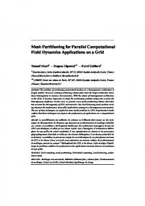
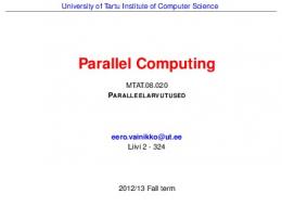
The Renater5 Network provides 10Gb/s dark fibre links that Grid’5000 utilizes for its inter-site communication network (Courtesy of www.renater.fr) . . . . . . . . . . . . . . . . . . . The architecture share of the top500 list from 1993 to 2010. (Courtesy of www.top500.org) . . . . . . . . . . . . . . . . . . A basic schematic of the IBM Cell processor showing one Power Processing Element (PPE) and eight Synergistic Processing Elements (SPEs). (Figure from NASA High-End Computing, Courtesy of Mercury Computer Systems, Inc.) . . . . A one-dimensional homogeneous (column-based) partitioning of a matrix with a total of nine partitions. . . . . . . . . . A two-dimensional homogeneous partitioning of a matrix with a total of nine partitions. . . . . . . . . . . . . . . . . . . A two-dimensional homogeneous partitioning of a matrix with a total of nine partitions showing pivot rows and columns and the directions they are broadcast. . . . . . . . . . . A two-dimensional heterogeneous partitioning consisting of nine partitions . . . . . . . . . . . . . . . . . . . . . . . . . . . An example of a column-based partitioning of the unit square into 12 rectangles. The rectangles of the partitioning all make up columns, in this case three. . . . . . . . . . . . . . . . . . . An example of Algorithm 2.2, a column-based partitioning for a 3 × 3 processor grid. Two steps are shown: Partitioning the unit square into columns then independently partitioning those columns into rectangles. . . . . . . . . . . . . . . . . . . A grid based partitioning of the unit square into 12 partitions. An optional grid based partitioning returned by Algorithm 2.3. A cartesian partitioning of the unit square into 12 rectangular partitions. All partitions have no more than four direct neighbors: up, down, left, right. . . . . . . . . . . . . . . . . . HCL Cluster load, CPU, memory and network profiles for the year April 2010 - March 2011. . . . . . . . . . . . . . . . . Schematic of the HCL Cluster Network. . . . . . . . . . . . .

7 9

13 21 22

23 25

28

29 30 31

32 39 41 vii

3.3

3.4

3.5

4.1

4.2

4.3 4.4

4.5

5.1 5.2

5.3

5.4

A two cluster configuration of the HCL Cluster. By bringing up NIC1 and bringing down NIC2 on hcl01 - hcl08, and the opposite for hcl09 - hcl16, and enabling the SFP connection between the switches, two connected clusters of eight nodes each are formed. . . . . . . . . . . . . . . . . . . . . . . . . . . A hybrid configuration of the HCL Cluster. By bringing up NIC1 and NIC2 on hcl01 and hcl02, they form one cluster connected to both switches. By bringing up NIC1 and bringing down NIC2 for hcl03 - hcl09, and the opposite for hcl10 - hcl16, two more clusters are formed, one connected to Switch1 and one connected to Switch2. . . . . . . . . . . . . . A hierarchal configuration of the HCL Cluster. By bringing up NIC1 and NIC2 on hcl01 and hcl02, they form one cluster. By bring up NIC1 and bringing down NIC2 for hcl03 - hcl09, and the opposite for hcl10 - hcl16, two more clusters are formed. The only way that Clusters 2 and 3 can communicate is through Cluster 1. . . . . . . . . . . . . . . . . . . . . . . . . . A heterogeneous non-rectangular partitioning consisting of two partitions, one rectangular and one a non-rectangular polygon. . . . . . . . . . . . . . . . . . . . . . . . . . . . . . . . A rectangular (column-based) partitioning to solve Problem 4.2. This is the rectangular counterpart of the non-rectangular partitioning in Figure 4.3 . . . . . . . . . . . . . . . . . . . . . A non-rectangular partitioning to solve Problem 4.2. . . . . . Cˆ values for a number A plot of the average and minimum LB of processors (entities) p from 1 to 40 for the column based rectangular partitioning of Beaumont et al. (2001b). For each value p, 2,000,000 partition values si are randomly generated. Cˆ A plot of the average and minimum LB values for a number of processors (entities) p from 1 to 40 except p = 2 using the rectangular partitioning, and for p = 2, the non-rectangular partitioning. For each value p, 2,000,000 partition values si are randomly generated. . . . . . . . . . . . . . . . . . . . . . The Straight-Line Partitioning and communication steps required to carry out C = A × B. . . . . . . . . . . . . . . . . . . The Square-Corner Partitioning and communication steps required to carry out C = A × B. The square partition is located in a corner of the matrix. . . . . . . . . . . . . . . . . . . . . . The TVC for the Square-Corner and Straight-Line Partitionings with serial communication, in terms of cluster power (partition area) ratio. . . . . . . . . . . . . . . . . . . . . . . . . The TVC for the Hybrid Square-Corner for Serial Communications and Straight-Line Partitionings with serial communication, in terms of cluster power (partition area) ratio. . . . .

42

43

43

50

53 54

57

58 64

65

67

68

viii

5.5

5.6

5.7

5.8

5.9

5.10

5.11

5.12

5.13

5.14

5.15

5.16

The TVC for the dominant communication of the StraightLine and Square-Corner Partitionings utilizing parallel communications. . . . . . . . . . . . . . . . . . . . . . . . . . . . . The TVC for the Hybrid Square-Corner for Parallel Communications and Straight-Line Partitionings with parallel communication, in terms of cluster power (partition area) ratio. . Parallel Communications: The TVC for SCPs1 →s2 , SCPs2 →s1 , SLP and HSCP-PC, where SCPx→y is the TVC of the SCP from partition x to partition y. . . . . . . . . . . . . . . . . . . . . . A partitioning similar to the Square-Corner Partitioning and the communication steps required to carry out C = A × B. The square partition is located adjacent to one of the sides of the matrix. . . . . . . . . . . . . . . . . . . . . . . . . . . . . . A partitioning similar to the Square-Corner Partitioning and the communication steps required to carry out C = A × B. The square partition is not adjacent to any sides of the matrix. A plot of the SHP vs. TVC values for Square-Corner and Square-Corner-Like Partitionings (Figures 5.8 and 5.9), and the Straight-Line Partitioning on the unit square. For the Square-Corner and Square-Corner-Like Partitionings the va√ lue of s2 ∈ (0.1, 0.25, 0.5, 0.75, 0.9) is varied. For the Straight-Line Partitioning the number of partitions p ∈ (2, 4, 9) is varied. . . . . . . . . . . . . . . . . . . . . . . . . . . Four polygonal partitionings seen so far, along with their bounding rectangles. Partitions A and B have a TVC proportional to the SHP. C and D do not. All partitions have a TVC proportional to their I value, the total number of row and column interrupts. . . . . . . . . . . . . . . . . . . . . . . The Square-Corner Partitioning showing the area (hatched) of Cluster 1’s C matrix which is immediately calculable. No communication is necessary to calculate this area. This is possible because Cluster 1 already owns the areas of A and B necessary to calculate C (also hatched). . . . . . . . . . . . . . Average communication times for the Square-Corner and Straight-Line Partitionings using serial communications. Network bandwidth is 100Mb/s, N = 4, 500. . . . . . . . . . Average communication times for the Square-Corner and Straight-Line Partitionings using serial communications. Network bandwidth is 500Mb/s, N = 4, 500. . . . . . . . . . Average communication times for the Square-Corner and Straight-Line Partitionings using serial communications. Network bandwidth is 1Gb/s, N = 4, 500. . . . . . . . . . . . Average execution times for the Square-Corner and StraightLine Partitionings using serial communications. Network bandwidth is 100Mb/s, N = 4, 500. . . . . . . . . . . . . . . .

72

73

74

76

77

79

81

82

84

85

86

88

ix

5.17

5.18

5.19

5.20

5.21

5.22

5.23

5.24

5.25

5.26

5.27

5.28

5.29

5.30

5.31

Average execution times for the Square-Corner and StraightLine Partitionings using serial communications. Network bandwidth is 500Mb/s, N = 4, 500. . . . . . . . . . . . . . . . Average execution times for the Square-Corner and StraightLine Partitionings using serial communications. Network bandwidth is 1Gb/s, N = 4, 500. . . . . . . . . . . . . . . . . . Average communication times for the Square-Corner and Straight-Line Partitionings using parallel communications. Network bandwidth is 100Mb/s, N = 4, 500. . . . . . . . . . Average communication times for the Square-Corner and Straight-Line Partitionings using parallel communications. Network bandwidth is 500Mb/s, N = 4, 500. . . . . . . . . . Average communication times for the Square-Corner and Straight-Line Partitionings using parallel communications. Network bandwidth is 1Gb/s, N = 4, 500. . . . . . . . . . . . Average execution times for the Square-Corner and StraightLine Partitionings using parallel communications. Network bandwidth is 100Mb/s, N = 4, 500. . . . . . . . . . . . . . . . Average execution times for the Square-Corner and StraightLine Partitionings using parallel communications. Network bandwidth is 500Mb/s, N = 4, 500. . . . . . . . . . . . . . . . Average execution times for the Square-Corner and StraightLine Partitionings using parallel communications. Network bandwidth is 1Gb/s, N = 4, 500. . . . . . . . . . . . . . . . . . A two cluster configuration of the HCL Cluster. By bringing up NIC1 and bringing down NIC2 on hcl03 - hcl05, and the opposite for hcl06 - hcl08, and enabling the SFP connection between the switches, two homogeneous connected clusters of three nodes each are formed. . . . . . . . . . . . . . . . . . Average communication times for the Square-Corner and Straight-Line Partitionings utilizing parallel communication. Network bandwidth is 100Mb/s, N = 4, 500. . . . . . . . . . Average communication times for the Square-Corner and Straight-Line Partitionings utilizing parallel communication. Network bandwidth is 500Mb/s, N = 4, 500. . . . . . . . . . Average communication times for the Square-Corner and Straight-Line Partitionings utilizing parallel communication. Network bandwidth is 1Gb/s, N = 4, 500. . . . . . . . . . . . Average execution times for the Square-Corner and StraightLine Partitionings utilizing parallel communication. Network bandwidth is 100Mb/s, N = 4, 500. . . . . . . . . . . . . Average execution times for the Square-Corner and StraightLine Partitionings utilizing parallel communication. Network bandwidth is 500Mb/s, N = 4, 500. . . . . . . . . . . . . Average execution times for the Square-Corner and StraightLine Partitionings utilizing parallel communication. Network bandwidth is 1Gb/s, N = 4, 500. . . . . . . . . . . . . .

89

90

92

93

94

96

97

98

99

100

101

102

103

104

105 x

5.32

5.33

6.1 6.2 6.3 6.4

6.5 6.6 6.7

6.8

6.9 6.10

6.11

6.12 6.13

6.14

6.15

6.16

Average communication times for the Square-Corner and Straight-Line Partitionings utilizing parallel communications. Network bandwidth is 1Gb/s, N = 15, 000. . . . . . . . 107 Average execution times for the Square-Corner and StraightLine Partitionings utilizing parallel communications. Network bandwidth is 1Gb/s, N = 15, 000. . . . . . . . . . . . . . 108 Star and Fully Connected topologies for three clusters. . . . . A Straight-Line Partitioning for three clusters. . . . . . . . . . The Square-Corner Partitioning for three clusters. . . . . . . . A two-dimensional Straight-Line Partitioning and data movements required to carry out C = A × B on three heterogeneous nodes or clusters. . . . . . . . . . . . . . . . . . . . . . . The Square-Corner Partitioning and data movements necessary to calculate C = A × B. . . . . . . . . . . . . . . . . . . . Examples of non-Square-Corner Partitionings investigated. . The three possible star topologies for three clusters using the Straight-Line Partitioning and associated data movements. Labels refer to data movements in Figure 6.4. Volumes of communication are shown in Table 6.1. . . . . . . . . . . . . . The three possible star topologies for three clusters using the Square-Corner Partitioning and associated data movements. Labels refer to data movements in Figure 6.5. Volumes of communication are shown in Table 6.2. . . . . . . . . . . . . . The surface defined by Equation 6.11. The Square-Corner Partitioning has a lower TVC for z < 0. . . . . . . . . . . . . . A contour plot of the surface defined by Equation 6.11 at z = 0. For simplicity, s2 = s3 , but this is not a restriction of the Square-Corner Partitioning in general. . . . . . . . . . . . . . Cluster 1’s partition is (C1 ∪ C2 ∪ C3 ). The sub-partition C1 = A1 × B1 is immediately calculable—no communications are necessary to compute its product. . . . . . . . . . . . . . . . . Overlapping Communication and Computation from an execution-time point of view. . . . . . . . . . . . . . . . . . . . Demonstration that the Square-Corner Partitioning for three clusters with a 1:1:1 ratio is not possible, as this ratio forces s2 and s3 to overlap, which is not allowed by definition. s1 = s1A + s1B . . . . . . . . . . . . . . . . . . . . . . . . . . . . . . . Communication times for the Square-Corner and StraightLine Partitionings on a star topology. Relative speeds s1 + s2 + s3 = 100. . . . . . . . . . . . . . . . . . . . . . . . . . . . . Execution times for the Square-Corner, Square-Corner with Overlapping and Straight-Line Partitionings on the star topology. Relative speeds s1 + s2 + s3 = 100. . . . . . . . . . . . Communication times for the Square-Corner and StraightLine Partitionings on a fully connected topology. Relative speeds s1 + s2 + s3 = 100. . . . . . . . . . . . . . . . . . . . . .

111 112 113

114 115 116

118

120 122

123

126 126

127

129

130

131 xi

6.17

6.18

6.19

7.1 7.2

7.3

7.4

7.5

8.1 8.2 8.3 8.4 8.5

D.1 D.2

D.3 D.4 D.5 E.1

Execution times for the Square-Corner, Square-Corner with Overlapping and Straight-Line Partitionings on a fully connected topology. Relative speeds s1 + s2 + s3 = 100. . . . 132 Communication times for the Square-Corner and Rectangular Partitionings on a star topology. Relative speeds s1 + s2 + s3 = 100. . . . . . . . . . . . . . . . . . . . . . . . . . . . . . . . 134 Execution times for the Square-Corner, Square-Corner with Overlapping and Straight-Line Partitionings on a star topology. Relative speeds s1 + s2 + s3 = 100. . . . . . . . . . . . . 134 An MDEM workcell. From Tacconi and Lewis (1997). . . . . . Comparison of the total communication times for the squarecorner and straight-line partitionings for power ratios ranging from 1 : 1 − 6 : 1. Max-Plus MMM, N = 7, 000. . . . . . Comparison of the total execution times for the square-corner and straight-line partitionings for power ratios ranging from 1 : 1 − 6 : 1. Max-Plus MMM, N = 7, 000. . . . . . . . . . . . . Comparison of the communication times for the MDEM DES model for both the Square-Corner and Straight-line Partitionings, N = 7, 000. . . . . . . . . . . . . . . . . . . . . . . . . . Comparison of the total execution times for the MDEM DES model for both the square-corner and straight-line partitionings, N = 7, 000. . . . . . . . . . . . . . . . . . . . . . . . . .

141

142

143

145

145

Examples of non-Square-Corner Partitionings investigated. . 147 An example of a four partition Square-Corner Partitioning . . 148 An example of a multiple partition Square-Corner Partitioning 148 An example of a rectangular matrix with one rectangular (α × β) partition and one polygonal (x × y − α × β) partition. . . . 150 The necessary data movements to calculate the rectangular matrix product C = A × B on two heterogeneous clusters, with one square and one polygonal partition per matrix. . . . 153 HCL Cluster load, CPU, memory and network profiles for the year April 2010 - March 2011. Provided by Ganglia. . . . HCL Cluster Load Report April 2010 - March 2011. Note that the load on hcl08, hcl11 and hcl12 is not lower than the other nodes. The scale of the y-axes of these graphs are affected by a very high 1 minute load in July. Provided by Ganglia. . . . HCL Cluster CPU Report April 2010 - March 2011. Provided by Ganglia. . . . . . . . . . . . . . . . . . . . . . . . . . . . . . HCL Cluster Memory Report April 2010 - March 2011. Provided by Ganglia. . . . . . . . . . . . . . . . . . . . . . . . . . HCL Cluster Network Report April 2010 - March 2011. Provided by Ganglia. . . . . . . . . . . . . . . . . . . . . . . . . . STREAM Benchmark Results for HCL Cluster, August 2010.

168

170 171 173 174 176

xii

NOTATION AND ABBREVIATIONS

AlgorithmXy→z

TVC for Algorithm X from partition y to partition z

DES

Discrete Event Simulation

HSCP-PC

Hybrid Square-Corner Paritioning using Parallel Communications

HSCP-SC

Hybrid Square-Corner Paritioning using Serial Communications

HSLP-PC

Hybrid Straight-Line Paritioning using Parallel Communications

HSLP-SC

Hybrid Straight-Line Paritioning using Serial Communications

LB

Lower Bound (Sum of Half Perimeters)

MDEM

Matrix Discrete Event Model

MMM

Matrix Matrix Multiplication

MPA

Max-Plus Algebra

N

Size of N × N matrix (number of rows and columns)

p

Number of partitions in a partitioning or number of computing entities (processors/clusters/etc.) mapped to partitions in a one-to-one mapping

ρ

When p = 2, the ratio of fastest entity to slowest entity, proportional to area of largest partition to smallest partition

s1 , s2 , . . . s p

Individual partition labels (or partition areas or speeds which are proportional to one another) of a particular partitioning, in non-increasing order

SCP

Square-Corner Partitioning

ˆ SHP (C)

Sum of Half Perimeters xiii

SLP

Straight-Line Partitioning

TVC

Total Volume of Communication

TVC AlgX

Total Volume of Communication for Algorithm X

xiv

THEOREMS/PROPOSITIONS AND PROOFS

5.1

Theorem: For all power ratios r greater than 3, the SquareCorner Partitioning has a lower TVC than that of the StraightLine Partitioning, and therefore all known partitionings, when p = 2 . . . . . . . . . . . . . . . . . . . . . . . . . . . . . . . . . . . . . . . . . . . . . . . . . . . . . . . . 63 Proof of Theorem 5.1 . . . . . . . . . . . . . . . . . . . . . . . . . . . . . . . . . . . . . . . .

5.2

Theorem: The TVC of the Square-Corner Partitioning, C is minimized only when the Square-Corner Partitioning assigns a square partition to the smaller partition area α × β = s2 . . . . . . 63 Proof of Theorem 5.2 . . . . . . . . . . . . . . . . . . . . . . . . . . . . . . . . . . . . . . . .

8.1

63

Proposition: Γ = α × y + β × x is minimized when the dimensions of the rectangular partition β × α is scaled to the matrix x α . . . . . . . . . . . . . . . . . . . . . . . . . . . . . . . . . . . . . . . 151 x × y such that = β y Proof of Proposition 8.1 . . . . . . . . . . . . . . . . . . . . . . . . . . . . . . . . . . . . . .

8.2

63

151

Proposition: The TVC, n × (α + β), for a multiplication of three rectangular matrices C = A × B is minimized when α = β, that is when the partition of area α × β is a square, provided α = β < m, n, p where A has dimensions m × n, B has dimensions n × p and C has dimensions m × p . . . . . . . . . . . . . . . . . . . . . . . . . . . 154 Proof of Proposition 8.2 . . . . . . . . . . . . . . . . . . . . . . . . . . . . . . . . . . . . . .

154

xv

LIST OF EQUATIONS

4.1 4.2 4.3

SHP of non-rectangular partitioning (Figure 4.3): 2 + x + y . √ SHP of SCP (Figure 4.3): 2 + 2 × s2 . . . . . . . . . . . . . . . . . . . . . . .

53 54

4.4

Condition for the SCP SHP to be less than the rectangular SHP √ (Figure 4.3): 2 + 2 × s2 < 3 . . . . . . . . . . . . . . . . . . . . . . . . . . . . . . 54 p √ LB, of the SHP (Any partitioning), Cˆ : 2 × ∑i=1 si . . . . . . . . . 56

5.1

TVC of SCP:

5.2

General form of Equation 5.1:

2×N×

√

s2 . . . . . . . . . . . . . . . . . . . . . . . . . . . . . . . . . .

62

α× N +β× N ..............

63

5.3

Restraints to Equation 5.2: α × β = s2 , 0 < α ≤ N, 0 < β ≤ N

63

5.4

For p = 2:

lim TVCSLP = N 2 . . . . . . . . . . . . . . . . . . . . . . . . . . . . . .

66

5.5

Optimality of SCP:

lim TVCSCP = 0 . . . . . . . . . . . . . . . . . . . . . . .

66

5.6

s2 in terms of ρ:

...................................

69

5.7

For p = 2:

70

5.8

For p = 2:

TVCSLP 1→2 = (1 − s2 ) × N 2 . . . . . . . . . . . . . . . . . . .   ρ TVCSLP 1→2 ∝ 1+ρ . . . . . . . . . . . . . . . . . . . . . . . . . . .

5.9

For p = 2:

70

5.10

For p = 2:

5.11

For p = 2:

5.12

For p = 2:

lim TVCSLP = N 2 . . . . . . . . . . . . . . . . . . . . . . . . . . . . . . √ √ TVCSCP 1→2 = 2 × s2 × (1 − s2 ) × N 2 . . . . . . . q  1 1 TVCSCP 1→2 ∝ 2 × .............. 1+ ρ − 1+ ρ   TVCSCP 2→1 ∝ 1+2 ρ . . . . . . . . . . . . . . . . . . . . . . . . . . .

5.13

Dominant communication (amongst SCP 1→2 and SCP 2→1 ) for hany q given ρ for  the  SCP i parallel communications: max 2 ×

ρ→∞

ρ→∞ s2 = 1+1 ρ

ρ→∞

1 1+ ρ

− 1+1 ρ ,

2 1+ ρ

............................

5.15

lim TVCSCP = 0 . . . . . . . . . . . . . . . . . . . . . . ρh→∞ h q   ii ρ 1 1 2 TVC of HSCP-PA: min 1+ρ , max 2 × 1+ ρ − 1+ ρ , 1+ ρ

5.16

SHP of SCP:

5.14

Optimality of SCP:

√ Cˆ = 2 × N + 2 × s2 . . . . . . . . . . . . . . . . . . . . . . . . .

70

70 70 71

71 72 73 77 xvi

√

s2 = √N

5.17

s2 in terms of ρ and N:

5.18

Total number of row and coloum interrupts, I, in any polygop nal partitioning: ∑i=1 (ri + ci ) . . . . . . . . . . . . . . . . . . . . . . . . . . . . 80

6.1

TVC for any rectangular partitioning:

112

6.2

Lower Bound of Equation 6.1:

112

6.3

TVC of the SLP for three partitions, showing q in Figure 6.2 (the only variable quantity): N 2 + N × q . . . . . . . . . . . . . . . . . . 113

6.4

Re-expression of Equation 6.3 : N 2 + s2 + s3 . . . . . . . . . . . . . . .

114

6.5

TVC of the SLP for three partitions (star network): N 2 + 2 × ( s2 + s3 ) . . . . . . . . . . . . . . . . . . . . . . . . . . . . . . . . . . . . . . . . . .

114

TVC of the SCP for three partitions (star network): √ √ 2 × N × ( s2 + s3 ) . . . . . . . . . . . . . . . . . . . . . . . . . . . . . . . . . . . . . . .

115

6.6 6.7 6.8 6.9

......................

ρ +1

p Cˆ = ∑i=1 (hi + wi ) . . p √ LB = 2 × ∑i=1 ai . . . . . . . . .

77

Restriction on relative speeds of entities for the SCP on three clusters: ss21 × ss31 ≤ 14 . . . . . . . . . . . . . . . . . . . . . . . . . . . . . . . . . . . . . . 116 √ √ TVC of SCP (star topology): ( s2 + s3 ) < 1.5 − s1 . . . . . . . 117 √ √ Rearrangement of Equation 6.8: z = ( s3 + s2 ) − 1.5 + s1 117

6.10

TVC of SCP is lower than SLP (fully-connected topology) √ √ when: ( s2 + s3 ) < 1 − s21 . . . . . . . . . . . . . . . . . . . . . . . . . . . . . . 121

6.11

Rearrangement of Equation 6.8 (Plotted in Figures 6.8 and √ √ 6.9): z = ( s2 + s3 ) − 1 + s21 . . . . . . . . . . . . . . . . . . . . . . . . . . . . 121

6.12

TVC for any rectangular partitioning (three partitions): p Cˆ = ∑i=1 (hi + wi ) = 3 + q . . . . . . . . . . . . . . . . . . . . . . . . . . . . . . . . . .

124 124

6.14

Lower bound of Equation 6.12: √ √ √ p √ LB = 2 × ∑i=1 si = 2 × ( s1 + s2 + s3 ) . . . . . . . . . . . . . . . √ √ TVC of SCP (three partitions): Cˆ = 2 + s2 + s3 . . . . . . . . .

6.15

For the SCP, p = 2:

lim Cˆ = 2 . . . . . . . . . . . . . . . . . . . . . . . . . . .

124

7.1

Max-Plus Algebra ⊕ and ⊗ operators:

6.13

7.3

de f =

a+b ......................

138

Definition of the Max-Plus Algebra: Rmax = (Rmax , ⊕, ⊗, e, e) . . . . . . . . . . . . . . . . . . . . . . . . . . . . . . . . . . .

140

Matrix Discrete Event Model State Equation: x = Fv × overlinevc + Fr × r c + Fu × u + FD × v D . . . . . . . . . . . .

140

v s = Sv × x . . . . . . . . . . . . . . . . . . . . . . .

140

a⊕b 7.2

de f =

s2 + s3 →0

124

max ( a, b) and a ⊗ b

7.4

MDEM Start Equation:

7.5

MDEM Resource Release Equation:

r s = Sr × x . . . . . . . . . . .

140

7.6

MDEM Product Output Equation:

y = Sy × x . . . . . . . . . . . . .

141

xvii

Γ = α×y+β×x ...............

150

α × β = (α − c) ( β + c0 ) . . .

151

α × n + β × n = n × (α + β) . . . . .

153

8.1

(Used in Proposition 8.1)

8.2

(Used Proof of Proposition 8.1)

8.3

(Used in Proposition 8.2)

xviii

PROBLEMS

4.1

The Matrix Partitioning Problem . . . . . . . . . . . . . . . . . . . . . . . . . . . . .

51

4.2

The General Matrix Partitioning Problem . . . . . . . . . . . . . . . . . . . .

51

xix

ALGORITHMS

2.1 2.2

2.3

Optimal column-based partitioning of a unit square between p heterogeneous processors . . . . . . . . . . . . . . . . . . . . . . . . . . . . . . . . . . . .

27

An optimal partitioning of a unit square between p heterogeneous processors arranged into c columns, each of which is made of r j processors where j ∈ {1, . . . , c} . . . . . . . . . . . . . . . . . . . . 28 Optimal grid-based partitioning of a unit square between p heterogeneous processors . . . . . . . . . . . . . . . . . . . . . . . . . . . . . . . . . . . . . . 30

2.4

Find r and c such that p = r × c and (r + c) is minimal (SubAlgorithm of Algorithm 2.3) . . . . . . . . . . . . . . . . . . . . . . . . . . . . . . . . . 31

2.5

Find a Cartesian partitioning of a unit square between p processors of a given shape p = r × c . . . . . . . . . . . . . . . . . . . . . . . . . . . . 33

4.1

An algorithm to solve Problem 4.2, the General Matrix Partitioning Problem, for p = 2 . . . . . . . . . . . . . . . . . . . . . . . . . . . . . . . . . . . 52

5.1

The Square-Corner Partitioning, a solution to Problem 4.2, the General Matrix Partitioning Problem, for p = 2 . . . . . . . . . . . . . . . 62

xx

DEFINITIONS

4.1

Rectangularity of a partitioning problem whose solution is to partition the unit square . . . . . . . . . . . . . . . . . . . . . . . . . . . . . . . . . . . . . 50

4.2

Non-Rectangularity of a partitioning problem whose solution is to partition the unit square . . . . . . . . . . . . . . . . . . . . . . . . . . . . . . . . 51

xxi

Dedicated to Catherine, the love of my life... and more...

ABSTRACT

The current state and foreseeable future of high performance scientific computing (HPC) can be described in three words: heterogeneous, parallel and distributed. These three simple words have a great impact on the architecture and design of HPC platforms and the creation and execution of efficient algorithms and programs designed to run on them. As a result of the inherent heterogeneity, parallelism and distribution which promises to continue to pervade scientific computing in the coming years, the issue of data distribution and therefore data partitioning is unavoidable. This data distribution and partitioning is due to the inherent parallelism of almost all scientific computing platforms. Cluster computing has become all but ubiquitous with the development of clusters of clusters and grids becoming increasingly popular. Even at a lower level, high performance symmetric multiprocessor (SMP) machines, General Purpose Graphical Processing Unit (GPGPU) computing, and multiprocessor parallel machines play an important role. At a very low level, multicore technology is now widespread, increasing in heterogeneity, and promises to be omnipresent in the near future. Scientific computing is undergoing a paradigm shift like none other before. Only a decade ago most high performance scientific architectures were homogeneous in design and heterogeneity was seen as a difficult and somewhat limiting feature of some architectures. However this past decade has seen the rapid development of architectures designed not only to exploit heterogeneity but architectures designed to be heterogeneous. Grid and massively distributed computing has led the way on this front. The current shift is moving from these to architectures that are not heterogeneous by definition, but heterogeneous by necessity. Cloud and exascale computing architectures and platforms are not designed to be heterogeneous as much as they are heterogeneous by definition.

xxiii

Indeed such architectures cannot be homogeneous on any large (and useful) scale. In fact more and more researchers see heterogeneity as the natural state of computing. Further to hardware advances, scientific problems have become so large that the use of more than one of any of the above platforms in parallel has become necessary, if not unavoidable. Problems such as climatology and projects including the Large Hadron Collider necessitate the use of extreme-scale parallel platforms, often encompassing more than one geographically central supercomputer or cluster. Even at the core level large amounts of information must be shared efficiently. One of the greatest difficulties in solving problems on such architectures is the distribution of data between the different components in a way that optimizes runtime. There have been numerous algorithms developed to do so over the years. Most seek to optimize runtime by reducing the total volume of communication between processing entities. Much research has been conducted to do so between distinct processors or nodes, less so between distributed clusters. This thesis presents new data partitioning algorithms for matrix and linear algebra operations (these algorithms would in fact work for any application with similar communication patterns). In practice these partitionings distribute data between a small number of computing entities, each of which can have great computational power themselves. These partitionings may also be deployed in a hierarchical manner, which allows the flexibility to be employed in a great range of problem domains and computational platforms. These partitionings, in hybrid form, working together with more traditional partitionings, minimize the total volume of communication between entities in a manner proven to be optimal. This is done regardless of the power ratio that exists between the entities, thus minimizing execution time. There is also no restriction on the algorithms or methods employed on the clusters themselves locally, thus maximizing flexibility. Finally, most heterogeneous algorithms and partitionings are designed by modifying existing homogeneous ones. With this in mind the ultimate goal of this thesis is to demonstrate that non-traditional and perhaps unintuitive algorithms and partitionings designed with heterogeneity in mind from the start can result in better, and in many cases optimal, algorithms and partitionings for heterogeneous platforms. The importance of this given the current outlook for, and trends in, the future of high performance scientific computing is obvious. xxiv

ACKNOWLEDGEMENTS

First I would like to most genuinely thank my advisor Dr. Alexey Lastovetsky whom I would like to nominate as the most capable, caring, and understanding supervisor ever to walk the face of planet Earth. I also owe many thanks to Prof. Joe Carthy, head of Computer Science and Informatics at UCD, for his help and understanding. Without Alexey and Joe, this thesis would not have ever reached fruition. I would like to thank Dr. Olivier Beaumont and Prof. M. Tahar Kechadi for agreeing to be my external and internal examiners respectively and taking the time to read my thesis and attend my viva, especially Olivier for travelling from France to Dublin. From the bottom of my heart I thank my mother Sharon—for everything. For understanding. For being there no matter what. For what we share. To say more would be tarnishing and dishonorable. I also specially thank my father Art, and stepmother Joann for everything they have given me, taught me, and for believing in me. I am forever indebted and grateful. Thank you. Thanks to my brother Wes for always being himself and keeping it real, and my sister-in-law Allison for the same. To my grandfather Art “Popa” who is the reason why I still scour parking lots for nails and screws so people don’t get flat tires, and my grandmother Joan “Nana” for always reminding me who to look out for. Thanks to my stepsisters Kristin and Andrea—I wish I saw you guys more. Thanks to my Uncle Bob and Caroline for knowing what it’s like and “what it is”. I would like to express a special thanks to my aunt Carol for too much to state, xxv

but especially for instilling the inspiration to travel in me, for without which I wouldn’t be here writing this. I would also like to thank all of the Beckers and the entire Finch Clan. It goes without saying that I thank my best friend, confidant, comrade, brother in arms, and partner in crime, Patrolman Tommy McAnney. His acknowledgement is mentioned for completeness and not out of necessity. Without Tommy I would not be even a close semblance to my present self, for better or worse, and whom I hope continues to impact my life until the day I die. I wish him and Sandra the best on their new baby Noelle, my niece—no matter how far away I am. I would also like to thank (in no particular order as always) my friends Carrie Hamblin, Donal Holohan, Dale Parsons, Eddie Pritsch, Marc Maggio, Tom Danza, Dave Marshall, Justin Smyth, Liam Power MSc. and his wife Gillian, Dr. John Regan and his wife Marylee, Dr. Mike Townsend and the soon to be Dr. Emma Howard, Dr. Mark “The Doctor” Dukes, and Dr. Fergus Toolan. Thanks to UCD staff who have helped me along the way: Patricia Geoghegan, Clare Comerford, Paul Martin, Tony O’Gara and Gerry Dunnion. I would also like to thank Dr. Gianluca Polastri, Dr. Joe Kiniry, and Dr. Nicola Stokes for their support over the years. A warm thanks to my UCD HCL colleagues Dr. Ravi Reddy, Dr. Thomas Brady, Dr. Michele Guidolin, Dr. Rob Higgins, Dr. Vladimir Rychov, Dr. Maureen O’Flynn, Dr. Xin Zuo, David Clarke and Kiril Dichev. I am greatly appreciative for the help of Rob, Vladimir, Dave and Kiril for taking over the administration of my “baby”, the HCL Cluster, and for initiating HCL Cluster 2.0—the first major upgrade since I built her. A very special thanks to my GCD friends and colleagues: Eamonn Nolan, Dr. Waseem Akhtar, Orla Butler, Dr. Faheem Bukhatwa, Dr. Kevin Casey, Eoin Carroll, Ruairi Murphy, Dr. Kevin Hely, once more Dr. Fergus Toolan, and the rest of the GCD Computing Science lecturers and staff. Thank you to the staff of the Drew University Department of Mathematics and Computer Science, Prof. Steve Kass and Prof. Christopher Van Wyk. And of course, the Drew University Physics Department, Prof. Robert Fenstermacher (Dr. F), Prof. James Supplee, and Prof. David McGee. Thank you to the ever changing but constantly vigilant crew of the F/V Mary M. and many people in the microcosms that are the Atlantic City Surf Clam xxvi

Fleet, and the Great Bay/Tuckerton Bay/Little Egg Harbor Baymen. Another very special thanks to Catherine’s patient, understanding, and loving family: Dr. David and Margaret Mooney, Ruth and Darbs, Deborah and Angus, and their beautiful families. I also would like to thank a very special group of people, some mentioned above—others not—who all went out of their way to help me in time of need. Thanks again—you know who you are. Finally I would like to—and will do—more than thank Dr. Catherine Mooney for her love, trust, perseverance, faith, and not least of all for saving my life. Sincerely yours, to all. - brett

Official Acknowledgements: This work was supported by the University College Dublin School of Computer Science and Informatics. This work was supported by Science Foundation Ireland. Experiments presented in this paper were carried out using the Grid’5000 experimental testbed, being developed under the INRIA ALADDIN development action with support from CNRS, RENATER and several Universities as well as other funding bodies. The author would like to thank Dr. Mark Dukes of the University of Iceland (at time of writing), now of the University of Strathclyde, for useful suggestions and emails (often not replied to) which always kept me going, and for getting me wrapped up in this Ph.D. business in the first place. The author would like to thank Ms. Sharon Becker and Dr. Fergus Toolan for proofreading and Dr. Catherine Mooney for proofreading and many useful insights.

xxvii

CHAPTER

ONE

INTRODUCTION “I would never have got to know this remote and beautiful island otherwise.” – Erwin Schrödinger, November, 19601

1.1

Motivation

Two general areas have provided the motivation for this work—those which are fundamental to this research, and the current state-of-the-art of high performance scientific computing. Areas which fall into the fundamental area include: What happens when we want to solve a well-established homogeneous problem on heterogeneous platforms? How can the performance of these problems be improved? Why have these problems, running on heterogeneous platforms, been largely ignored by research groups? Where is scientific computing headed in the future? Platforms and architectures which are central to the state-of-the-art and future of scientific computing include: • Super Computing • Grid Computing 1 Schrödinger,

E. (1967). What is life? With mind and matter and autobiographical sketches. Cambridge University Press.

1

• Cloud Computing • Cluster Computing • GPGPU Computing • Multicore Computing

1.1.1

Fundamentals

This work started with a simple question. Take two heterogeneous processing elements—how can they work together to best solve a specific problem? This question immediately raised many more. What happens if we add another element to make three? What about four? Is there something specific about the problems we want to solve that can be exploited to improve performance? How will the data partitioning and distribution impact the communication and execution times? How will the communication network affect the communication times? How will this affect execution times? Regardless of the answers to these questions, two things are certain. It is desired for these elements to balance the computational load between themselves optimally, and to communicate data necessary for computations optimally. Unfortunately optimality is not always possible. These two tasks often turn out to be surprisingly difficult on heterogeneous platforms. Indeed solutions to problems that prove to be optimal on heterogeneous platforms are rare. Often some of the most simple tasks on homogeneous platforms turn out to be NP-Complete when attempted on heterogeneous ones (Beaumont et al., 2002a). Sometimes approximation algorithms are found, often heuristics and problem restrictions are resorted to, and in some cases not even theoretical results exist. In the latter case researchers have deemed it necessary to resort to experimental approaches for reproducibility and comparison studies. Tools to facilitate such have already been developed (Canon and Jeannot, 2006). To answer our questions we choose as a testbed the problem of matrix matrix multiplication (MMM). Matrices are probably the most widely used mathematical objects in scientific computing and their multiplication (or problems reducible to MMM) appear very frequently in all facets of scientific computing (Dongarra and Lastovetsky, 2006). Indeed, MMM is the prototype of tightlycoupled kernels with a high spatial locality that need to be implemented efficiently on distributed and heterogeneous platforms (Beaumont et al., 2001b). Moreover most data partitioning studies mainly deal with matrix partitioning. 2

Why would we want to extend MMM to heterogeneous platforms? As stated in Beaumont et al. (2001b), the future of computing platforms is best described by the keywords distributed and heterogeneous. Our fundamental motivation stems from two sources. First, there exist many general heterogeneous MMM algorithms which work well for several, dozens, hundreds, or even thousands of nodes, but all currently known algorithms result in simple, perhaps naïve partitionings when applied to the architecture of a small number of interconnected heterogeneous computing entities (two, three, etc.). Examples of these methods are explored in Beaumont et al. (2001b, 2002b); Dovolnov et al. (2003); Kalinov and Lastovetsky (1999); Lastovetsky (2007). As stated earlier we intentionally set out to investigate the particular case of a small number of computing entities to see what is happening in what is sometimes perceived to be a “degenerate” case. Despite its existence for at least 30 years, parallel MMM research has almost completely ignored this area. Early work is presented in Becker and Lastovetsky (2006, 2007), and some early application results in Becker and Lastovetsky (2010). Second, we at the Heterogeneous Computing Laboratory2 are keenly aware of the parallel, distributed and especially the heterogeneous nature of computing platforms which are omnipresent in scientific computing, and that most parallel and distributed algorithms in existence today are designed for, and only work efficiently on homogeneous platforms. After discussing the aforementioned load balancing and communication issues, we will survey modern scientific computing platforms, and where parallelism, distribution and heterogeneity impact them. 1.1.1.1

Load Balancing

The issue of load balancing is well studied and well understood, but not without its challenges. For a detailed study see Boulet et al. (1999). Neglecting the obvious such as the nature of the problem itself, failures and fluctuating capability due to other outside influences or factors, the issue can be reduced to a knowledge of the problem and the computing elements themselves. Suppose there is an amount of work W to do. If element A is capable of doing a work x in time t1 and element B is capable of doing a work y in time t2 , the problem can be statically partitioned quite easily. We know that A works at a y speed s1 = tx1 and B works at a speed s2 = t2 . If we normalize the speeds so 2 hcl.ucd.ie

3

that s1 + s2 = 1, element A is to receive an amount of work equal to W × s1 and element B is to receive an amount of work equal to W × s2 . Theoretically this would result in A and B finishing their work partitions in the same time, thus being optimal from a load balancing point of view. For homogeneous computing elements such a problem scales well. In fact homogeneous systems are a standard platform for many supercomputers today (See 1.1.2). Current supercomputers utilize thousands of homogeneous elements (normally nodes or processors) working in parallel. At the time of writing the fourth fastest computer on Earth is “Kraken”, a Cray CT5 Family, XT5-HE System Model, with 16,488 AMD x86_64 Opteron Six Core processors running at 2,600 MHz (a total of 98,928 cores) at the National Institute for Computational Sciences/University of Tennessee in Tennessee, USA.3 Kraken is capable of 1,028,851 GFlops. For reference the laptop I am writing on now is an Intel Core Duo T5500 running at 1.66Ghz with 2GB memory, and has a peak performance of around 1Gflop, depending on the benchmark. An embarrassingly parallel problem—that is a problem that can be cut into any number of pieces as small as one wants with little or no communication between processes—could be theoretically balance load by partitioning the problem into 98,928 partitions and have each core solve one of the partitions. This would theoretically solve the whole problem in about one millionth of the time it would take my laptop. This is of course neglecting an multitude of factors such as data distribution and re-collection times, architectural differences, and vast memory and storage issues. 1.1.1.2

Communication

It is the communication aspects of data partitioning and distribution which make designing such algorithms difficult. Again ignoring faults, other nonrelated network traffic, etc., does the communication component of data partitioning affect the time it takes to solve the problem? How is it affected? what are these effects? Are there possibilities of deadlocks, race conditions and other parallel communication issues? Most fundamentally, two simple questions arise: • How does the way we partition the data affect the execution time? • What is the best way to partition the data so that we minimize the com3 www.nics.tennessee.edu/computing-resources/kraken

4

munication time, thus (hopefully) minimizing the execution time? These questions can be quite difficult to answer—sometimes impossible to answer—but can have a significant effect on the overall execution time.

1.1.2

State-of-the-art Scientific Computing

1.1.2.1

The Top500

The website www.top500.org maintains a list of the fastest computers on Earth, updated bi-annually. The fastest computer on Earth at the time of writing is “Jaguar”, a Cray XT5-HE At Oak Ridge National Laboratory in Tennessee, USA.4 Jaguar is composed of two physical partitions (not to be confused with data partitions). The first partition is “XT5” with 37,376 Opteron 2435 (Istanbul) processors running at 2.6GHz, with 16GB of DDR2-800 memory, and a SeaStar 2+ router with a peak bandwidth of 57.6Gb/s. The resulting partition contains 224,256 processing cores, 300TB of memory, and a peak performance of 2.3 petaflop/s (2.3 quadrillion floating point operations per second). The second partition “XT4” has 7,832 quad-core AMD Opteron 1354 (Budapest) processors running at 2.1 GHz, with 8 GB of DDR2-800 memory (some nodes use DDR2-667 memory), and a SeaStar2 router with a peak bandwidth of 45.6Gb/s. The resulting partition contains 31,328 processing cores, more than 62 TB of memory, over 600 TB of disk space, and a peak performance of 263 teraflop/s (263 trillion floating point operations per second). The routers are connected in a 3D torus topology for high bandwidth, low latency, and high scalability. The combined top500 benchmarked performance is 2,331,000 GFlops. For interest, 2,331,000 GFlops is 2.27 times faster than Kraken, and significantly over two million times faster than the computer I am using at the moment. What makes Jaguar different to Kraken? Jaguar is heterogeneous. Note that this is not necessarily the reason that Jaguar is faster, it is just a fact. Actually, the second and third fastest, along with the sixth and seventh fastest computers on Earth are heterogeneous. That makes half of the ten fastest computers on Earth heterogeneous. Jaguar is heterogeneous in processor architecture, speed, number of cores per processor, memory, storage, and network communications. 4 www.nccs.gov/computing-resources/jaguar/

5

We have seen that heterogeneity has pervaded the area of supercomputers, however there are several other cutting-edge technologies emerging that are inherently heterogeneous. 1.1.2.2

Grid Computing

Grid Computing has become very popular for high performance scientific computing in recent years (Foster and Kesselman, 2004). Compared to standalone clusters and supercomputers, grids tend to be more loosely coupled, geographically dispersed, and are inherently heterogeneous. Unlike some clusters, grids tend to be built with general purpose scientific computing in mind. In short, grids seek to combine the power of multiple clusters and/or sites to solve problems. Grid computing has been sought and promoted by organizations such as CERN5 to analyze the vast amounts of data that such bodies produce. A primary advantage of grid computing is that each constituent cluster or site can be built from off-the-shelf commodity hardware that is cheaper to purchase, upgrade and maintain. Additionally there has been a major effort to produce middleware—software which makes the management of resources and jobs easier and cheaper than a custom solution. For an example, see SmartGridRPC, a project between the HCL and the University of Tennessee (Brady et al., 2010). The primary disadvantage is the geographic distribution of sites which combined with commodity network hardware makes inter-site communication much slower than the often custom-built, very expensive networks of supercomputers. An example of an existing grid is Grid’5000 (Bolze et al., 2006). Located in France, Grid’5000 is composed of nine sites. Porto Alegre, Brazil has just become the official tenth site, and Luxembourg is expected to join soon. There is also a connection available which extends to Japan. Grid’5000 has 1,529 nodes from Altix, Bull, Carri, Dell, HP, IBM and SUN. A total of 2,890 processors with a total of 5,946 cores from both AMD and Intel. Local network connections are Myrinet, Infiniband, and Ethernet. All Grid’5000 sites in France are connected with a 10Gb/s dark fibre link provided by RENATER (The French National Telecommunication Network for Technology Education and Research)6 . Figure 1.1 Shows the backbones of the Renater 5 public.web.cern.ch/public/ 6 www.renater.fr

6

Figure 1.1: The Renater5 Network provides 10Gb/s dark fibre links that Grid’5000 utilizes for its inter-site communication network (Courtesy of www.renater.fr) Network which connects the sites of Grid’5000. The important aspect of this figure is the architecture of the network connecting the various sites across France, and the connections to sites outside France. In keeping with the decentralized nature of grid computing, Grid’5000 is funded by INRIA (The French National Institute for Research in Computer Science and Control)7 , CNRS (The French National Centre for Scientific Research)8 , the universities of all sites, and some regional councils. This highlights another advantage of grids—the cost of building and maintaining them can be shared amongst many different bodies easily. 7 www.inria.fr 8 www.cnrs.fr

7

A total of 606 experiments are listed on the Grid’5000 website as completed or in progress. A tiny sample of experiment areas include genetic algorithms, task scheduling, middleware testing, modeling physical phenomena, and linguistic processing. As an example of Grid’5000 performance, the Nancy site has a 92 node Intel Xeon cluster which achieves 7,360 GFlops, and a 120 node Intel Xeon cluster, which achieves 1,536 GFlops. As the Nancy site is average (actually a little lower than average) in size for Grid’5000, we can roughly calculate the power by dividing Nancy’s power by the number of nodes at Nancy then multiplying by the total number of nodes in Grid’5000. This roughly equals 65,000 Gflops, or 36 times slower than Jaguar. This of course is just a rough Gflop count, and does not take any specific parameters into account. 1.1.2.3

Cloud Computing

Cloud computing can have a different definition, depending on the source. Generally it is a form of computing where not only the details of who, what and where a user’s computations are being carried out are hidden from the user, but perhaps even the knowledge and details of how to calculate the computations. The general idea is that a user supplies data to a client program or interface, along with either a full program or program description, and the client program then selects the proper, available servers—which can be anywhere on the globe—and gets the work carried out. When the computation is complete, the results are delivered back to the user. For some applications where there are “canned” solutions available, all the user will have to do is supply the data and specify what solution is desired. In effect all the user needs to do is specify the problem and the solution will be delivered. In most definitions the “cloud” is a metaphor for the Internet, as one could view cloud computing as the computational (number crunching) equivalent of the Internet we know today. All the user knows is to open a web browser, supply information (what they’re looking for) and the results come back. The user doesn’t know from who, or where, and doesn’t care—it just comes. 1.1.2.4

Cluster Computing

In 1982 Sun Microsystems was founded upon the motto “The Network is the Computer”. This philosophy paved the way for the popularization of cluster computing, largely through their software products. At the time computer operating systems were designed only to run on and exploit the power of 8

stand-alone computers. Sun’s operating systems were revolutionary in that they were designed to harness the power of networks of computers. Two or more such computers working together to achieve a common goal constitute a cluster. The topic itself, and much research focusing specifically on cluster computing as a pure subject is quite old, dating back 30 or more years. In fact such systems first started out as “the poor man’s supercomputer” in academic departments where researchers would leave jobs running perhaps all night instead of purchasing expensive supercomputer time (Beaumont et al., 2001b). Top500 Architecture Share 1993−2008

00000000000000000000 11111111111111111111 500 000000000000000000000000000 00000000000000000000 11111111111111111111 111111111111111111111111111

Year

111 000 000 Cluster 111 000 111 000 111 111 000 000 MPP 111 000 111 000 111 111 000 000 All Others 111 000 111 000 111

2010

1993

Number of Systems

00000000000000000000 11111111111111111111 111111111111111111111111111 000000000000000000000000000 00000000000000000000 11111111111111111111 000000000000000000000000000 111111111111111111111111111 00000000000000000000 11111111111111111111 000000000000000000000000000 111111111111111111111111111 00000000000000000000 11111111111111111111 000000000000000000000000000 111111111111111111111111111 00000000000000000000 11111111111111111111 000000000000000000000000000 111111111111111111111111111 00000000000000000000 11111111111111111111 000000000000000000000000000 111111111111111111111111111 00000000000000000000 11111111111111111111 000000000000000000000000000 111111111111111111111111111 00000000000000000000 11111111111111111111 000000000000000000000000000000 111111111111111111111111111111 000000000000000000000000000 111111111111111111111111111 00000000000000000000 11111111111111111111 000000000000000000000000000000 111111111111111111111111111111 000000000000000000000000000 111111111111111111111111111 00000000000000000000 11111111111111111111 000000000000000000000000000000 111111111111111111111111111111 000000000000000000000000000 111111111111111111111111111 00000000000000000000 11111111111111111111 000000000000000000000000000000 111111111111111111111111111111 000000000000000000000000000 111111111111111111111111111 00000000000000000000 11111111111111111111 000000000000000000000000000000 111111111111111111111111111111 000000000000000000000000000 111111111111111111111111111 00000000000000000000 11111111111111111111 000000000000000000000000000000 111111111111111111111111111111 000000000000000000000000000 111111111111111111111111111 00000000000000000000 11111111111111111111 000000000000000000000000000000 111111111111111111111111111111 000000000000000000000000000 111111111111111111111111111 00000000000000000000 11111111111111111111 000000000000000000000000000000 111111111111111111111111111111 000000000000000000000000000 111111111111111111111111111 00000000000000000000 11111111111111111111 000000000000000000000000000000 111111111111111111111111111111 00000000000000000000 11111111111111111111 000000000000000000000000000000 111111111111111111111111111111 00000000000000000000 11111111111111111111 000000000000000000000000000000 111111111111111111111111111111 00000000000000000000 11111111111111111111 000000000000000000000000000000 111111111111111111111111111111 00000000000000000000 11111111111111111111 000000000000000000000000000000 111111111111111111111111111111 000000000000000000000000000000 111111111111111111111111111111 000000000000000000000000000000 111111111111111111111111111111 000000000000000000000000000000 0 111111111111111111111111111111

Figure 1.2: The architecture share of the top500 list from 1993 to 2010. (Courtesy of www.top500.org) Cluster Computing has since become the dominant architecture for all scientific computing, including top500 supercomputers. Figure 1.2 shows the architectures of top500 computers from 1993 to 2010. In 1993 no top500 computers were clusters. They were MPPs, constellations, SMPs, and others—even single processor vector machines. It wasn’t until the late 1990s that the first clusters joined the top500, but their popularity exploded, largely due to low cost and simple maintenance combined with great power. By 2007 about 80% of top500 machines were clusters and the number has grown to the point today where almost all top500 machines are clusters. Let us demonstrate the prevalence and importance of clusters in the context of this section. Although not comprehensive in terms of state-of-the art scientific computing, this does provide a good overview: 9

• Top500 - Almost all computers in the top500 are based on cluster platforms • Grid Computing - All grids are geographically distributed clusters or clusters of clusters. • Cloud computing - As the name implies, how clusters fit in is slightly “fuzzy” but surely any cloud of even a moderate size would include clusters. • GPGPU (General Purpose Graphical Processing Unit) computing is done on clusters of GPU machines. • Multicore computing physically exists at the processor (single machine) level, but it is clusters of multicores which make up many top500 machines and grids. Thus we have seen quite simply that cluster computing is actually the foundation of all other types of computing discussed here. 1.1.2.5

GPGPU (General Purpose Graphical Processing Unit) Computing

Another exciting area of high performance computing in which interest is gathering great pace is using Graphics Processing Units (GPUs) alongside traditional CPUs. Traditionally GPUs are used to take the burden of, and accelerate the performance of, rendering graphics (today often 3D graphics) to a display device. To this end, GPUs have evolved to become in most cases quite specialized in the operations necessary to do so, namely linear algebra operations. This makes them quite unintentionally well suited for many high performance scientific applications, as many of these rely heavily or exclusively on linear algebra operations. Examples of problems which have been explored with this approach include oil exploration, image processing and the pricing of stock options (Kruger and Westerman, 2005). Beyond the confines of linear algebra, interest has also been gathering in so called General Purpose Computing on Graphics Processing Units or (GPGPU). This seeks to harness the computing power of GPUs to solve increasingly general problems. Recently nVidia and ATI (by far the two largest GPU manufacturers) have joined with Stanford University to build a dedicated GPU-based

10

client for the Folding@home project which is one of the largest distributed computing projects in the world. Briefly, Folding@home9 harnesses (mostly) the unused CPU cycles of home computers across the globe to perform protein folding simulations and other molecular dynamics problems. A user downloads a client application and then when the user’s computer is idle, packets of data from a server at Stanford are downloaded, and processed by the client program. Once the data has been processed using the client, the results are sent back to the server and the process repeated. At the time of writing the total number of active CPUs on the project is 286,723 with a total participation of 5,514,891 processing units, 343,843 of which are GPUs, and 1,003,463 are PlayStation 3s running the Cell Processor.10 The total power of the Folding@home project is estimated to be 2,958,000 Gflops, theoretically 1.27 times faster than Jaguar. We must keep in mind however that if a problem with the complexity, memory, and data dependencies of those being solved on Jaguar was given to the Folding@home network, it would be incredibly—actually uselessly—slow, and very, very difficult to program. Nonetheless, Folding@home is surely an example of extreme heterogeneity. Of course, mixed in those millions of computers are Linux, MAC, and Windows machines as well. The power of such a distributed, heterogeneous “system” can only be effectively harnessed due to the nature of the problems that are being solved. Although extremely large, the problems are embarrassingly parallel. In this case the key is that there are no data dependencies. No user computer needs information from, or needs to send information to, any other user computer. Further, the order in which data is sent back to the server does not matter. As long as all of the results eventually come back, they can be reconstructed back to the original order. If some results don’t come back (which is inevitable), the data necessary to get the results are simply farmed out to another active user. Nonetheless we see a system with the power of a supercomputer, using a heterogeneous hierarchy at every level—client/server, system, processor and core. For another similar project, see SETI@home11 , which distributes data from the Aricebo radio telescope in Puerto Rico to home users’ computers, which then analyze the data for signs of extra-terrestrial life. 9 http://folding.stanford.edu 10 fah-web.stanford.edu/cgi-bin/main.py?qtype=osstats 11 setiathome.ssl.berkeley.edu

11

To wrap up GPU processing, nVidia has announced a new configuration using their video cards. Their PhysX physics engine can now be used on two heterogeneous nVidia GPUs in one machine.12 A physics engine is software that computes and replicates the actual physics of events in real-time to make computer graphics more realistic such as shattering glass, trees bending in the wind, and flowing water. In this configuration the more powerful GPU renders graphics while the other is completely dedicated to running the PhysX engine. 1.1.2.6

Multicore Computing

At a much lower level, multicore technology has become mainstream for most computing platforms from home through high-performance. Multicore processors have more than one core, which is the element of a processor that performs the reading and executing of an instruction. Originally processors were designed with a single core, however a multicore processor can be considered to be a single integrated circuit with more than one core, and can thus execute more than one instruction at any given time. Embarrassingly parallel problems can approach a speedup equal to the number of cores, but a number of limiting factors including the problem itself normally limits such realization. Currently most multicore processors have two, four, six or eight cores. The number of cores possible is limited however, and is generally accepted to be in the dozens. More cores would require more sophisticated communication systems to implement and are referred to as many-core processors. The Cell processor is a joint venture between Sony Corporation, Sony Computer Entertainment, IBM, and Toshiba and has nine cores. One core is referred to as the “Power Processor Element” or PPE, and acts as the controller of the other eight “Synergistic Processing Elements” or SPEs. See Figure 1.3 for a basic schematic of the processing elements of the Cell processor. The PPE can execute two instructions per clock cycle due to its multithreading capability. It has a 32KB instruction and 32KB L1 cache, and a 512KB L2 cache. The PPE performance is 6.2 GFlops at 3.2GHz. Each SPE has 256KB embedded SRAM and can support up to 4GB of local memory. Each SPE is capable of a theoretical 20.8 GFlops at 3.2GHz. Recently IBM has shown that the SPEs can reach 98% of their theoretical peak performance using optimized parallel matrix matrix multiplication.13 The elements are connected by an Element Interconnect Bus 12 www.nvidia.com/object/physx\_faq.html\#q4 13 www.ibm.com/developerworks/power/library/pa-cellperf/

12

Figure 1.3: A basic schematic of the IBM Cell processor showing one Power Processing Element (PPE) and eight Synergistic Processing Elements (SPEs). (Figure from NASA High-End Computing, Courtesy of Mercury Computer Systems, Inc.) (EIB), with a theoretical peak bandwidth of 204.8GB/s. The Sony PlayStation 3 is an example of the Cell processor at work. To increase fabrication yields, Sony limited the number of operational SPEs to seven. One of the SPEs is reserved for operating system tasks, leaving the PPE and six SPEs for game programmers to use. Clearly this has utilized the Cell to create a more heterogeneous system. This is exemplary of a truly heterogeneous system in practice—functionality can be arranged as desired, and needed. The Cell processor is used in the IBM “Roadrunner” supercomputer, which is a hybrid of AMD Opteron and Cell processors and is the third fastest computer on Earth (formerly number 1) at 13,752,776 GFlops. The PlayStation 3 “Gravity Grid” at the University of Massachusetts at Dartmouth Physics Department is a cluster of sixteen Playstation 3 consoles used to perform numerical simulations in the areas of black hole physics such as binary black hole coalescence using perturbation theory.14 Clearly the Cell processor is an example of parallel heterogeneous computing at a very low-level, with very diverse applications, and introduces a hierarchy with the PPE controlling the SPE’s, while also maintaining some number crunching abilities itself. The future of heterogeneous multicore architectures is expanding rapidly. The 14 arxiv.org/abs/1006.0663

13

past month alone has seen two major developments. First, a research team at the University of Glasgow has announced what is effectively a 1000 core processor, although it differs from a traditional multicore chip as it is based on FPGA technology, which could easily lend itself to heterogeneous use. Second, the release of the first multicore mobile phones has been announced. The natural need for heterogeneity in such platforms is discussed in van Berkel (2009).

1.1.3

Heterogeneity

We have seen that heterogeneity and hierarchy have infiltrated every aspect of computing from supercomputers to GPUs, Cloud Computing to individual processors and cores. We have also seen that in many, many ways all of these technologies are interwoven and can join to form hybrid entities themselves. To conclude it is fitting to state that homogeneity (even if explicitly designed) can be very difficult and expensive to maintain, and easy to break (Lastovetsky, 2003). Any distributed memory system will become heterogeneous if it allows several independent users to simultaneously run applications on the same system at the same time. In this case different processors will inevitably have different workloads at any given time and provide different performance levels at different times. The end result would be different performances for different runs of the same application. Additionally, network usage and load, and therefore communication times will also be varied with the end result being different communication times for a given application, further interfering with the delivery of consistent performance for the same application being run more than once. Component failure, aging, and replacement can all also impact homogeneity. Are identical replacement components available? Are they costly? Do all components deliver uniform and consistent performance with age? Even if these problems are managed, eventually when upgrading or replacement time comes, all upgrades and replacements must be made at the same time to maintain homogeneity. We see now that heterogeneity is the natural state of parallel and distributed systems. Most interestingly, vendors are now starting to intentionally design and construct systems and platforms for high performance scientific computing which are heterogeneous from the outset. This is perhaps a natural progression as specialized hardware and software aimed at one particular class

14

of problem is desired over more general-purpose approaches that yield poor performance.

1.2

Objectives

The main goal of this thesis is to present, validate, and experimentally demonstrate a new partitioning algorithm for high performance scientific computing on parallel hierarchal heterogeneous computing platforms. This partitioning could theoretically be deployed on any heterogeneous architecture including all those discussed in Section 1.1.2. It will also be shown that this partitioning can serve as the basis for other new partitionings. The following is a list of other goals that will and must be realized along the way. First the state-ofthe-art will be reviewed, before the underlying mathematical principles of this new partitioning are explored. For the cases in which it applies the partitioning will be discussed and it’s optimality proven. A hybrid algorithm will be discussed which is designed to be optimal in all cases for certain problem domains. The construction of a heterogeneous cluster hand-designed specifically for problems discussed in this thesis will be detailed. The partitioning will be compared to the state-of-the-art and both its benefits and deficits discussed. The partitioning will be modelled, simulated, and then experimentally verified before being shown to be beneficial to application areas indicative of those widely in use today. Then, future directions of research will be presented. Finally, as stated, most heterogeneous algorithms and partitionings are designed by modifying existing homogeneous ones. The ultimate goal of this thesis is to demonstrate the concept that unintuitive, non-traditional algorithms and partitionings, designed with heterogeneity in mind from the start, can result in better—and optimal—algorithms and partitionings for high performance computing on heterogeneous platforms.

1.3

Outline

Chapter 2: Background and Related Work In this section existing research in the area of heterogeneous parallel data partitioning and matrix matrix multiplication is explored. The state-of-the-art is clearly described and the benefits and drawbacks of current techniques are detailed. 15

Chapter 3: UCD Heterogeneous Computing Laboratory (HCL) Cluster This chapter describes the design and construction of a heterogeneous cluster specifically for the simulation and testing of heterogeneous algorithms and partitionings. The cluster is unique in its ability to be configured in network parameters and topology which allows for testing on any number of heterogeneous scenarios. Chapter 4: Partitioning a Matrix in Two – Geometric Approaches This chapter presents and mathematically validates a new data partitioning method for matrix matrix multiplication on heterogeneous networks. A geometrical approach is used to present the design of the partitioning. The partitioning is shown to be optimal in most cases, and a hybrid partitioning is proposed which would be optimal in all cases. Chapter 5: The Square-Corner Partitioning This chapter defines the Square-Corner Partitioning and its application to matrix matrix multiplication. The optimality of the partitioning as well as other benefits such as overlapping computation and communication are explored. Experimental results are presented, first on two processors, then on small groups of clusters, then on two larger clusters. Chapter 6: The Square-Corner Partitioning on Three Clusters In this chapter the Square-Corner Partitioning is extended to three clusters. Both topologies possible (fully-connected and star) are explored. Experimental results are given for simulations on three processors and three clusters. Results of overlapping computation and communication are also explored. Chapter 7: Max-Plus Algebra and Discrete Event Simulation on Parallel Hierarchal Heterogeneous Platforms This chapter presents the results of applying the Square-Corner Partitioning on Max-Plus Algebra operations and a Discrete Event Simulation Application. Chapter 8: Moving Ahead – Multiple Partitions and Rectangular Matrices This chapter presents work on extending partitionings to more than three and to non-square matrices. The Square-Corner Partitioning is shown to be useful for the multiplication of rectangular matrices in particular. Chapter 9: Conclusions and Future Work In this chapter overall conclusions of this work are drawn, and indications of exciting areas of future work are detailed.

16

CHAPTER

TWO

BACKGROUND AND RELATED WORK 2.1

Data Distribution and Partitioning

In 1997, van de Geijn and Watts noted: “It seems somewhat strange to be writing a paper on parallel matrix multiplication almost two decades after commercial parallel systems first became available. One would think that by now we would be able to manage such an apparently straight forward task with simple, highly efficient implementations. Nonetheless, we appear to have gained a new insight into this problem” (van de Geijn and Watts, 1997). It is now 2010 and researchers across the globe are still working with great ferocity on parallel matrix multiplication algorithms! This chapter presents a summary of parallel matrix multiplication, first and briefly on homogeneous algorithms, then heterogeneous algorithms. We start with the homogeneous case because most heterogeneous algorithms are modifications of their homogeneous counterparts. We will of course end with the current state-of-the-art in heterogeneous parallel MMM algorithms. In order to discuss these algorithms however, we must discuss data distribution and therefore data partitioning, which is the focus of this thesis. The partitioning of data directly affects the communication between processing elements. These communications may be over a super-fast bus between cores or long-distance copper or fibre networks, but either way it is typically communications that are an order of magnitude or more slower than processing speed and therefore the most significant bottleneck in parallel and distributed algorithms.

17

2.2

Introduction

As stated in the summary, it is now 2010 and we are still working with great ferocity on parallel matrix multiplication algorithms. This is due to the common thread that ran through the motivation in Section 1.1.2, from cloud computing with theoretically millions or more machines at work, through supercomputers with hundreds of thousands of processors, down to multicore chips on single machines. This thread is heterogeneity. In fact there was another common thread, distribution, which is due to necessary physical separation of computing elements. Be they two computers on opposite sides of the Earth, or two cores separated by hundredths of a centimeter, computing elements need to be physically separated and therefore must communicate to work together. This brings up an interesting question—Why must processing elements be physically separated? There are many answers to this question, the main reasons being: (i) Heat. Too many processing elements in too small a space creates too much heat which increases cooling costs in the best case, and in the worst case leads to component failure. (ii) Cost. Along with cooling cost, communication hardware costs are perhaps the largest cost factors. The ultra-fast communication buses between cores and processors and main-memory are simply too expensive to scale up. In fact such devices only barely scale out of the micro and into the macro scales. It is much, much cheaper to connect machines with commodity, off-the-shelf communication hardware, than two processors with an ultra-fast motherboard bus that is metres or more long. (iii) Convenience. For economical, social and other reasons, it makes sense to distribute computing resources geographically. In the case of the Folding@home project introduced in the motivation, the utilized resources were already geographically distributed, and then exploited. We also saw that there are computing resources, particularly grids (for example Grid’5000 (Bolze et al., 2006)), that are intentionally built to be geographically distributed. This is not done due to pure physical necessity, but to make cost, maintenance, upgrading and logistics more convenient. (iv) Modularity and Reliability. Closely related to convenience is the modularity and reliability of the system itself. If a supercomputer was just a 18

single, massive processor (if physically feasible), what would happen if it or a crucial component failed? Everything would grind to a halt. What happens if a chip, node, or even an entire cluster or even in the extreme an entire site in Grid’5000 goes down? All other processors, nodes, clusters, and sites go merrily on with their business. This gets even better if the middleware can handle fault tolerance. The user may not realize that a component failed, other than a possibly longer execution time, but not necessarily, and what counts most is the results will still be correct. (v) “That’s just the way it is” or ‘‘That’s just the way things evolve”. Everything from beings with exoskeletons to animals with internal skeletons, from dinghies to the most massive cargo ships, from subatomic particles to the most massive of stars have a physical size limit per entity. At some point the only way to generate more beings, carrying capacity, or energy, is to make more of them. And thanks to quantum physics no two things can occupy the same space at the same time, so more things means more space which necessitates physical distribution. There are certainly more parameters, especially when individual cases are examined. Perhaps one more question could be asked, particularly in reference to (i) and (ii) above. Why can’t a chip be manufactured which is just one big chip? Let’s ignore heat, cost, reliability and other obvious answers and instead of answering the question directly just render the question itself a moot point. If it were possible to do so we would still be dealing with communications. Communications between individual registers or even in the extreme, transistors on the chip itself, still need to be done optimally or at least efficiently. Again, as in Section 1.1 we see that communication between different entities is an inherent fact of computing, no matter what scale we are dealing with and no matter how we look at or abstract the issue.

2.3

Parallel Computing for Matrix Matrix Multiplication

Currently parallel computing is undergoing a paradigm shift. It is spreading from supercomputer centers which have been established utilizing specialized, often custom-built and terribly expensive computers which are used and programmed by highly trained and specialized people to clusters of off-the19

shelf commodity workstations that (with the proper libraries and some skill) can be used by “ordinary” people. By ordinary I mean people whose primary profession need not be programming supercomputers. Such clusters have already pervaded academia and industry, but promise to do so further, and are now becoming accessible to and “toys” of home users, who desire to use them. Indeed these clusters remain the poor man’s supercomputer (Csikor et al., 2000) as discussed in the motivation. Cloud Computing promises to carry this concept even further, with additional abstraction, and less expertise needed by the user. From this point forward we will not consider heterogeneity (or homogeneity for that matter) and communication to be exclusive. From one follows the other. Any parallel architecture (homogeneous or heterogeneous) without some communication somewhere is useless. Let’s just talk about parallel computing for a while. We will start with the simple case, homogeneous parallel computing. In this thesis I exclusively address the linear algebra kernel of Matrix-Matrix Multiplication (MMM) as the prototype problem for High Performance Parallel Computing on Heterogeneous Networks (with the exception of some application areas explored later in Chapter 7). This is a common and justifiable decision as matrices are probably the most widely used mathematical objects in scientific computing (Lastovetsky, 2007). Further to that, MMM is the prototype for a group of tightly coupled kernels with a high special locality that should be implemented efficiently on parallel platforms [both homogeneous and heterogeneous] (Beaumont et al., 2001b). Throughout this thesis, if only one matrix is being discussed, it may be thought of as the product C of two other matrices A and B, such that C = A × B. In these cases, A and B are partitioned identically to C. This has become a standard in the field.

2.3.1

Data Partitioning for Matrix Matrix Multiplication on Homogeneous Networks

The problem of matrix partitioning on homogeneous networks has been well studied. It has perhaps been studied to exhaustion with the exception of the inclusion of application specific issues, or particular hardware/software considerations. In other words the theoretical underpinnings have been established and are very unlikely to undergo a significant change. For more see Kumar et al. (1994). 20

Figure 2.1: A one-dimensional homogeneous (column-based) partitioning of a matrix with a total of nine partitions. Let us start then with homogeneous matrix partitioning for three reasons: 1. Because it is well established

2. Because most heterogeneous algorithms are designed either from, or at least with, their homogeneous counterparts in mind

3. It is often the homogeneous counterparts that heterogeneous algorithms are compared to, particularly to address their effectiveness or lack thereof (Lastovetsky and Reddy, 2004) When partitioning a matrix for distribution between homogeneous processors1 , the problem of load balancing is easy, as all processors have equal speed, and therefore each partition will have equal area. Thus the issue quickly turns to minimizing communications. The simplest homogeneous partitioning of a matrix is in one dimension, with the matrix partitioned into either rows or columns of equal area as in Figure 2.1. The other way to accomplish a homogeneous partitioning is to use a two-dimensional partitioning, which results in a grid of partitions as in Figure 2.2. 1 We

begin by talking about partitioning and distribution among individual processors and later will scale this up to individual clusters. Entity will sometimes be used to refer to any unit capable of processing be it a core, processor, cluster, etc.

21

Figure 2.2: A two-dimensional homogeneous partitioning of a matrix with a total of nine partitions. Let us start with the two-dimensional case. We have a matrix multiplication C = A × B and for simplicity we make each a square n × n matrix. Assume we have p homogeneous processors P1 , P2 , . . . , Pp . Again for simplicity let us assume that the processors are arranged in a grid of size p1 × p2 = p such that p1 = p2 . In this case the processors and the partitions of the matrix overlay each other exactly such that at each step k, • Each processor Pi,k , i ∈ . . . p1 broadcasts horizontally ai,k to processors Pi,∗ • Each processor Pk,j , j ∈ . . . p2 broadcasts vertically bk,j to processors P∗,j This allows each processor Pi,j to update its portion of C, using ci,j = ci,j + ai,k × bk,j . In other words, at each step of the algorithm each processor does the following: • Each processor broadcasts the part of the pivot column which it owns horizontally to the processors in the same processor row which the processor resides in • Each processor broadcasts the part of the pivot row which it owns vertically to the processors in the same processor column which the processor resides in. This is shown in Figure 2.3. 22

11 00 00 11 00 11 00 11 00 11 00 11 00 11 00 11 00 11 00 11 00 11 00 11 00 11 00 11 00 11 00 11 00 11 00 11 00 11 00 11 00 11 00 11 00 11 00 11 00000000000000000000000 11111111111111111111111 00 11 00000000000000000000000 11111111111111111111111 00 11 00000000000000000000000 11111111111111111111111 00 11 00 11 00 11 00 11 00 11 00 11 00 11 00 11 00 11 00 11 00 11 00 11 00 11 00 11 00 11 00 11 00 11 00 11 00 11

Figure 2.3: A two-dimensional homogeneous partitioning of a matrix with a total of nine partitions showing pivot rows and columns and the directions they are broadcast. The popular ScaLAPACK library uses this technique, but uses a blocked version (Blackford et al., 1997). In this case, each matrix element (say Ci,j , Ai,j , and Bi,j ) is a square r × r block. For each processing entity there will be an optimal value of r, depending on memory and other architecture-specific details. Usually the number of blocks d(n/r )e × d(n/r )e is greater than the number of processors p1 × p2 . In this case the blocks are distributed in a cyclic fashion so that each processor is responsible for updating several blocks of the C matrix at each step k. It is worth noting at this point that the total volume of communication (TVC) of the calculation described above is proportional to the sum of the half perimeters (SHP) of each partition. This can be viewed rather simply; at each step, each processor responsible for a square of x × x elements receives x elements from a row-mate and x elements from a column-mate for a total of 2x √ elements. Since the partitions are all equal in size and dimension (if p evenly divides n), the same will be true for all processors. Thus at each step each processor is receiving a number of elements proportional to 2 × x, the sum of each partition’s half perimeter. It is easy to show that the two-dimensional partitioning has a lower TVC than the one-dimensional partitioning. Given a fixed area, the rectangle covering that area and having the smallest perimeter is a rectangle that is square, and the fact that any other partitioning strategy would force at least one partition to be non-square, any other partitioning strategy (including the one-dimensional 23

partitioning described above) would result in a greater SHP, and therefore a greater TVC. There are other parallel algorithms for MMM, such as: • Cannon’s algorithm (Lee et al., 1997) • DNS (Kumar et al., 1994) • one-dimensional and two-dimensional Systolic (Golub and Van Loan, 1996) • Broadcast Multiply Roll (Fox et al., 1988) • the Transpose Algorithm (Lin and Snyder, 1992) • SUMMA (Scalable Universal Matrix Multiplication Algorithm (van de Geijn and Watts, 1997), which is used in PBLAS (the Parallel Basic Linear Algebra Subprograms) library (Choi et al., 1996) Each has its advantages and disadvantages and a discussion of each is beyond the scope of this thesis. They are mentioned for completeness.

2.3.2

Data Partitioning for Matrix Matrix Multiplication on Heterogeneous Networks

Now let us assume a heterogeneous network. We have p heterogeneous processors P1 , P2 , . . . , Pp , each free to run at a speed unique to all other processors. We will express these speeds relatively as s1 , s2 , . . . , s p . Similar to the homogeneous algorithm above at each time step k, there will be a pivot row broadcast vertically and a pivot column broadcast horizontally. These rows and columns can be either made of individual matrix elements or blocks of elements as described above. If we are discussing blocks, they will remain square for efficiency on a processor-local level. We will now see how a modification of the homogeneous algorithm above can lead to heterogeneous ones. The heterogeneity of processors means that we cannot necessarily partition the matrix into squares. We will generalize and partition the matrix into nonoverlapping rectangles. Similar to the homogeneous algorithm, data should be partitioned so that the area of each rectangular partition is proportional to the speed of the processor who owns it. From a load-balancing point of view it is only the area of the rectangles that matter. The dimensions of each rectangle 24

Figure 2.4: A two-dimensional heterogeneous partitioning consisting of nine partitions are free for us to choose. Figure 2.4 shows a heterogeneous partitioning of nine rectangles. The difficult question is this: What dimensions should each rectangle have to minimize the total inter-partition (and therefore inter-cluster, if each partition were owned by a cluster) volume of communication? Actually the word difficult turns out to be an understatement. This question (when formally defined) turns out to be NP-complete (Beaumont et al., 2002b). There is no known polynomial time solution to this question. In other words, for even modestly sized problems, unreasonable (or impossible) lengths of time would be needed to achieve an optimal solution. We must therefore resort to approximation algorithms or heuristics. Generally these begin by imposing a restriction or restrictions on the proposed solution to allow it to run in polynomial time. The next three subsections will explore the state-of-the-art in attempts to do so. Before we do it is worth mentioning (again for completeness) that we are and will be discussing static partitionings only. Static partitionings are determined based on input data, and after that the partitioning does not change throughout the course of the program. A dynamic partitioning is one that does (more properly has the ability to) change the initial partitioning before the program terminates. One way to do this is use the past to predict the future (Beaumont et al., 2001b). This method determines how to best change the partitioning based on how the program is commencing during execution. There also exist dynamic master-slave techniques. These all may suffer from various draw-

25

backs, not the least that they must be very general and therefore less likely to perform as well as static approaches which are tailored to a specific problem domain. 2.3.2.1

Restricting the General Approach: A Column Based Partitioning

In (Beaumont et al., 2001b) the authors state the general matrix partitioning problem: • Given p computing elements P1 , P2 , . . . , Pp , the relative speed of which is p

characterized by a positive constant Si , where

∑ Si = 1

i =1

• Partition a unit square into p rectangles so that – There is a one to one mapping of elements to rectangles – The area of the rectangle allocated to element Pi is equal to Si where i ∈ {1, . . . , p}. p

– The partitioning minimizes ∑ (wi + hi ), where wi is the width of the i =1

rectangle and hi is the height of the rectangle assigned to element Pi . Partitioning the unit square into rectangular partitions with areas proportional to the speed of the processing elements mapped to them is aimed at balancing the load of the work done by each processing element. As a rule there will be more than one partitioning satisfying this condition. p

Minimizing the sum of half-perimeters of the partitions,

∑ (wi + hi ) is aimed

i =1

at minimizing the total volume of communication between the elements. This is possible because with the problem of MMM, at each step, each processing element that does not own the pivot row and column receives an amount of data proportional to the half-perimeter of the rectangular partition it owns. Therefore the amount of data communicated at each step between all processing elements will be proportional to the sum of the half-perimeters of all partip

tions, ∑ (wi + hi ), less the sum of the heights of the partitions owning the pivot i =1

column, (one in the case of the unit square), and less the sum of the widths of the partitions owning the pivot row (also one for the unit square). Thus at each p

step the total data communicated will be

∑ (wi + hi ) − 2.

Because the total

i =1

26

amount of data communicated between the processing elements is the same at each step of the algorithm, the total amount of data communicated during the p

execution of the algorithm will also be proportional to

∑ (wi + hi ) − 2. There-

i =1

p

fore minimization of ∑ (wi + hi ) − 2 will minimize the total volume of commui =1

p

nication between all partitions. Clearly any solution minimizing p

will also minimize

∑ ( wi + h i )

i =1

∑ (wi + hi ) − 2.

i =1

The authors of (Beaumont et al., 2001b) have shown that this general partitioning problem is NP-Complete and therefore heuristics must be resorted to in order to find optimal solutions. Such a heuristic is presented by Beaumont et al. (2001b) which restricts the rectangles of the partitioning to forming columns such as in Figure 2.5. The algorithm follows: Algorithm 2.1 (Beaumont et al., 2001b): Optimal column-based partitioning of a unit square between p heterogeneous processors: • First, the processing elements are re-indexed in the non-increasing order of their speeds, s1 ≥ s2 ≥ . . . ≥ s p . The algorithm only considers partitionings where the i-th rectangle in the linear column-wise order is mapped to processor Pi , i ∈ {1, . . . , p}. • The algorithm iteratively builds the optimal c column partitioning β(c, q) q

of a rectangle of height 1 and width

∑ s j for all c ∈ {1, . . . , p} and q ∈

j =1

{c, . . . , p}: – β(1, q) is trivial. – For c > 1, β(c, q) is built in two steps: ∗ First, (q − c + 1) candidate partitionings { β j (c, q)}( j ∈ {1, . . . , q − c + 1}) are constructed such that β j (c, q) is obtained by combining the partitioning β(c − 1, q − j) with the straightforward partitioning of the last column (the column number q

c) of the width

∑

si into j rectangles of the corresponding

i = q − j +1

areas sq− j+1 ≥ sq− j+2 ≥ . . . ≥ sq . q − c +1

∗ Then, β(c, q) = β k (c, q) where β k (c, q) ∈ { β j (c, q) j=1 } and minimizes the sum of the half-perimeters of the rectangles. 27

Figure 2.5: An example of a column-based partitioning of the unit square into 12 rectangles. The rectangles of the partitioning all make up columns, in this case three. • The optimal column-based partitioning will be a partitioning from the p set { β(c, p)c=1 } that minimizes the sum of half-perimeters of rectangles. Algorithm 2.1 runs in O(p3 ) time. 2.3.2.2

A More Restricted Column-Based Approach

Kalinov and Lastovetsky (2001), further restrict the column-based geometrical partitioning by assuming that the processing elements are already arranged in a set of columns (i.e. assuming that the number of columns c in the partitioning and the mappings of rectangles in each column to the processors are given). The algorithm is as follows. Algorithm 2.2: (Kalinov and Lastovetsky, 2001): An optimal partitioning of a unit square between p heterogeneous processors arranged into c columns, each of which is made of r j processors where j ∈ {1, . . . , c}: • Let the relative speed of the i-th processor from the j-th column, Pi,j be c

si,j where

rj

∑ ∑ si,j = 1.

j =1 i =1

• First, partition the unit square into c vertical rectangular slices so that the 28

11111111 00000000 00000000 11111111 00000000 11111111 00000000 11111111 00000000 11111111 00000000 11111111 00000000 11111111 00000000 11111111 00000000 11111111 00000000 11111111 00000000 11111111 00000000 11111111 P_ 1 00000000 11111111 00000000 11111111 00000000 11111111 00000000 11111111 00000000 11111111 00000000 11111111 00000000 11111111 00000000 11111111 00000000 11111111 00000000 11111111 00000000 11111111

P_ 2

111111 000000 000000 111111 000000 111111 000000 111111 000000 111111 000000 111111 000000 111111 000000 111111 000000 111111 000000 111111 000000 111111 000000 111111 P_ 3 000000 111111 000000 111111 000000 111111 000000 111111 000000 111111 000000 111111 000000 111111 000000 111111 000000 111111 000000 111111 000000 111111

11111111 00000000 00000000 11111111 00000000 11111111 P11 00000000 11111111 00000000 11111111 00000000 11111111

11111111111 00000000000 00000000000 11111111111 00000000000 11111111111 P12 00000000000 11111111111 00000000000 11111111111 00000000000 11111111111 00000000000 11111111111

P21

P22

11111111 00000000 00000000 11111111 00000000 11111111 P31 00000000 11111111 00000000 11111111 00000000 11111111

11111111111 00000000000 00000000000 11111111111 00000000000 11111111111 00000000000 11111111111 P32 00000000000 11111111111 00000000000 11111111111 00000000000 11111111111 00000000000 11111111111

11111 00000 00000 11111 00000 11111 P13 00000 11111 00000 11111 00000 11111

P23 11111 00000 00000 11111 P33 00000 11111 00000 11111 00000 11111

Figure 2.6: An example of Algorithm 2.2, a column-based partitioning for a 3 × 3 processor grid. Two steps are shown: Partitioning the unit square into columns then independently partitioning those columns into rectangles. rj

width of the j-th slice w j =

∑ si,j .

i =1

– This partitioning makes the area of each vertical slice proportional to the sum of speeds of the processors in the corresponding column. • Second, each vertical slice is partitioned independently into rectangles in proportion to the speeds of the processors in the corresponding column. Algorithm 2.2 runs in linear time. Figure 2.6 shows this for a 3 × 3 processor grid. 2.3.2.3

A Grid Based Approach

Lastovetsky (2007) describes a partitioning which imposes a further restriction on the column-based approaches. The restriction is that the partitionings must form a grid as in Figure 2.7. This can be viewed from another approach. The grid based partitioning is one which partitions the unit square into rectangles so that there exist p and q such that any vertical line crossing the square will intersect exactly p rectangles and any horizontal line crossing the square will intersect exactly q rectangles, regardless of where these lines cross the unit square. It is proposed and proven in (Lastovetsky, 2007) that in the case of a unit square partitioned into a grid of c columns, each of which is partitioned into r rows, the sum of half-perimeters of all partitions will be equal to (r+c). The corollaries which precipitate from this is that the optimal grid based partitioning 29

Figure 2.7: A grid based partitioning of the unit square into 12 partitions. is one which minimizes r+c, and that the sum of half-perimeters of the optimal grid-based partitioning does not depend on the mapping of the processors onto the nodes of the grid. The algorithm for the optimal grid-based partitioning follows. Algorithm 2.3: (Lastovetsky, 2007): Optimal grid-based partitioning of a unit square between p heterogeneous processors: • Find the optimal shape r × c of the processor grid such that p = r × c and (r + c) is minimized. • Map the processors onto the nodes of the grid. • Apply Algorithm 2.2 of the optimal partitioning of the unit square to this r × c arrangement of the p heterogeneous processors. Step one finds the optimal shape of the processor grid that minimizes the sum of half-perimeters of any grid based partitioning for any mapping of the processors onto the nodes of the grid. Step two simply does the mapping (by any means). Step three then finds one such partitioning where the area of each rectangle is proportional to the speed of the processor owning it. It is noted that the solution is always column-based due to the nature of Algorithm 2.2. The first step of Algorithm 2.3 is described by Algorithm 2.4.

30

Figure 2.8: An optional grid based partitioning returned by Algorithm 2.3. Algorithm 2.4 (Lastovetsky, 2007): Find r and c such that p = r × c and (r + c) is minimal:

√ r = b pc while (r > 1) if (( p mod r ) == 0) goto stop; else r − −; stop: c = p/r Figure 2.8 shows an optimal grid based partitioning returned by algorithm 2.3. In (Lastovetsky, 2007) the correctness of these algorithms is proven and the complexity of Algorithm 2.4 is shown to be O(p3/2 ). Experimental results are also given which demonstrate the effectiveness of the grid based approach. 2.3.2.4

Cartesian Partitionings

The grid-based partitioning strategy is not the most restrictive partitioning problem that has been addressed. A Cartesian partitioning can be obtained from a column-based partitioning by imposing an additional restriction; namely that the rectangular partitionings also make up rows as seen in Figure 2.9. This results in any given partition having no more than four direct neighbors (up, down, left, right). 31

Figure 2.9: A cartesian partitioning of the unit square into 12 rectangular partitions. All partitions have no more than four direct neighbors: up, down, left, right. Cartesian partitionings are important in heterogeneous algorithm design due to their scalability. This is due to no partition having more than one neighbor in any given direction. This lends itself to a scalable partitioning for algorithms which have communication patterns which only involve nearest neighbors, or for that matter, communications only between partitions in the same row and/or column. Due to the additional restriction imposed by a Cartesian partitioning an optimal partitioning may not be achievable. The load between partitionings may not be perfectly balanced for some combinations of relative computing element speeds. This renders relative speeds unusable and the problem should be reformulated in terms of absolute speeds. The Cartesian partitioning problem can be formulated as follows: • Given p processors, the speed of each of which is characterized by a given positive constant, find a Cartesian partitioning of a unit square such that: – There is a one to one mapping of partitions to computing elements. ) ( max hi × w j , where hi is the height – The partitioning minimizes i,j sij of partitions in the i-th row, w j is the width of partitions in the j-th column, si,j is the speed of the computing element owning the j-th partition in the i-th row, where i ∈ {1, . . . , r }, j ∈ {1, . . . , c}, and p = r × c. 32

To the author’s knowledge the Cartesian problem has not been studied as stated above in general form. An algorithm to solve this problem has to find an optimal shape r × c of the computing element grid, the mapping of the elements onto the grid, and the size of the partitions allocated to the elements. Simplified versions of the problem have been studied however (Beaumont et al., 2001a; Dovolnov et al., 2003). If the shape r × c of the partitioning is given the problem is proven to be NP-Complete (Beaumont et al., 2001a). In addition it is not known if given both the shape r × c of the grid and the mapping of computing elements onto the grid are given, there exists a polynomial time solution. An approximate algorithm of the simplified Cartesian problem where the shape r × c is given in Algorithm 2.5. Algorithm 2.5 (Beaumont et al., 2001a): Find a Cartesian partitioning of a unit square between p processors of the given shape p = r × c: • Step 1. Arrange the processors so that if linearly ordered row-wise, beginning from the top left corner, they will go in a nonincreasing order of their speeds. • Step 2. For the processor arrangement, apply a known algorithm to find an approximate solution, {hi }ri=1 , {w j }cj=1 . • Step 3.Calculate the areas hi , wi of the rectangles of the partitioning. • Step 4. Rearrange the processors so that ∀i, j, k, l : sij ≥ skl ⇔ hi × w j ≥ hk × wl . • Step 5. If Step 4 does not change the arrangement of the processors then return the current partitioning and stop the procedure else go to Step2.

2.4

Conclusion

In this section we saw that communication is unavoidable in parallel computing. Normally this is thought of in terms of computer networks: wires, switches, routers, etc. However it must be realized that communication occurs even at lower levels than two geographically distributed clusters. It happens between machines in the same rack, and even between cores on a single processor. 33

We then examined how the partitioning of data, specifically in the case of matrix matrix multiplication, can affect the amount of data that needs to be communicated. After briefly looking at elementary one and two-dimensional partitionings, several state-of-the-art methods were explored including general two-dimensional cases, more restricted column-based approaches, even more restricted strategies such as grid based, and finally very restricted twodimensional approaches in cartesian cases. All of these partitioning strategies have two common threads. They all balance load and they all seek to minimize the sum of communication between partitions, normally through imposing restrictions. However this is not a hard rule, as in some cases relaxing restrictions can lead to better solutions.

34

CHAPTER

THREE

UCD HETEROGENEOUS COMPUTING LABORATORY (HCL) CLUSTER 3.1

Summary

The UCD Heterogeneous Computing Laboratory’s main cluster was designed and hand built by myself to provide a controllable heterogeneous test platform. The cluster serves to develop and run HCL software and as a testbed for applications that are to be deployed on larger systems. The cluster is composed of 16 compute nodes and two switches, along with the necessary peripherals (server/UPS/access node/etc.) The cluster is unique in two ways: the bandwidth between each node can be controlled from 8kb/s up to 1Gb/s, and that the cluster itself can be split into two clusters in several configurations. The compute nodes are heterogeneous in vendor, chipset, memory, operating system, number of cores, and many other ways. A complete host of scientific programming and monitoring system software is installed to allow HCL group members to easily develop and test applications. To date the cluster has been used in over 40 publications and six Ph.D. theses, with collaborators from many international universities. For a list see Appendix A. It has also been used for the development and testing of eight software packages. A list is included in Appendix B. A major upgrade (HCL Cluster 2.0) is currently under way in order to further serve the expanding needs of the Heterogeneous Computing Laboratory.

35

3.2

The UCD Heterogeneous Computing Laboratory Cluster

The UCD Heterogeneous Computing Laboratory’s main cluster1 is designed to provide a controllable hierarchal heterogeneous environment for research in high performance heterogeneous computing. The cluster was hand-built over the course of four months from purchasing to end of testing. It is completely stand-alone (that is to say it is not dependent on outside support, infrastructure, software, security, etc.). The cluster is housed in a 42U server rack with power backup supplied by an APC Smart 1500 UPS. The main server is heterogeneous.ucd.ie (heterogeneous). Domain Name Service is provided by BIND (Berkley Internet Name Daemon). NAT (Network Address Translation) is implemented between the external network and the internal network (the compute nodes). Clonezilla is used for recovery issues. All compute nodes and access/server machines are kept synchronized through NTP (Network Time Protocol). DHCP (Dynamic Host Configuration Protocol) is used to configure IP addresses and hostnames. NFS (Network File System) is used to allow compute nodes access to server files. NIS (Network Information Service) is used to organize user names and passwords across the cluster. Smartmontools provides backup services. TORQUE/PBS manages jobs that users submit to the queues. There are four queues, with varying priority and preemption policies: 1. normal, where most jobs (which should not be interrupted) are placed. It has the highest priority. 2. lowpri, for running jobs which may run for extended periods but are interruptible. Should a job A be placed on the normal queue while a lowpri job B is running, B will be sent a kill signal, so it may shut down cleanly, and then it will be re-queued on the system, so it can resume running after A has finished. 3. service, which is for running service jobs such as home directory backups. This has lower priority than the above queues and jobs running on this queue are preemptable. 4. volunteer, which has the lowest priority, and is for executing volunteer computing jobs during otherwise idle periods. These jobs are also 1 hcl.ucd.ie/hardware

36

preemptable. For security the only incoming connections allowed are ssh except requests originating from inside the cluster that require incoming packets such as http, NTP, etc. which are also allowed. Incoming ssh connections are only allowed if they originate from designated IP addresses: currently some user machines and a central UCD School of Computer Science server (csserver.ucd.ie). The only other machine that is allowed is a gateway machine (hclgate.ucd.ie), which again is completely under group control. This machine is used to allow connections from users outside the UCD Intranet should csserver be down. Security on this machine is kept to the highest standard and updates as it is connected to the outside Internet.

3.3

Software

The HCL Cluster has been outfitted with all current packages necessary for the group to carry out parallel heterogeneous program and software development. Software packages currently available on the cluster include the following: • autoconf

• evince

• automake

• fftw2

• ATLAS

• GDB

• autotools

• git

• BLAS

• gfortran

• Boost

• gnuplot

• C\C++ (gnu)

• Graphviz

• ChangeLog

• gsl-dev

• colorgcc

• LAPACK

• Dia

• LATEX

• doxygen

• libboost-graph-dev

• Eclipse

• libboost-serialization-dev 37

• libtool

• python

• logp_mpi

• qhull

• mc • MPI (MPICH, OpenMPI)

• R • r-cran-strucchange

• netperf • octave3.2 • openmpi-bin

• STL • subversion

• openmpi-dev

• valgrind

• OProfile

• vim

Software specifically for Heterogeneous Computing includes the following: • Parallel extension of C: – mpC • Extensions for MPI: – HeteroMPI – libELC • Extensions for GridRPC: – SmartGridSolve – NI-Connect • Computation benchmarking, modeling, dynamic load balancing: – FuPerMod – PMM • Communication benchmarking, modeling, optimization: – CPM – MPIBlib Software specifically for Mathematical Heterogeneous Computing includes the following: 38

• HeteroScaLAPACK • Hydropad Details on all of the above are available at: http://hcl.ucd.ie/wiki/index.php/Main\_Page and http://hcl.ucd.ie/wiki/index.php/HCL\_cluster. Ganglia is used to provide real-time cluster status to users and is available at: http://heterogeneous.ucd.ie/ganglia. Figure 3.1 shows overall cluster load, CPU, memory and network reports for the year April 2010 March 2011. For node by node load, CPU, memory and network reports, see Appendix D.

Figure 3.1: HCL Cluster load, CPU, memory and network profiles for the year April 2010 - March 2011.

3.4

Heterogeneity

The compute section of the cluster is comprised of 16 nodes (hcl01 - hcl16) from three different vendors (Dell, IBM, HP). It was designed to be heterogeneous in hardware, software, and network as follows.

3.4.1

Hardware

• Processor Architecture (Intel , AMD ) 39

• Processor Speed (1.8 - 3.6 GHz) • Ram (256 MB, 512 MB, 1GB) • Main Storage (SCSI, SATA), (80 - 240GB) • Front Side Bus (533, 800, 1k MHz) • L2 Cache (1, 2 MB)

3.4.2

Operating Systems

• MS Windows (current option) • Debian Linux “squeeze” kernel 2.6.32 (currently) • Fedora Linux / Debian Linux (formerly)

3.4.3

Network

An overall schematic of the HCL Cluster network is given in Figure 3.2. • 2 x Cisco 3560G 24+4 Switches (8Kb/s - 1Gb/s configurable bandwidth per port) The HCL cluster is unique in two ways which make it specifically and particularly suited for research in heterogeneous computing. First, the ingress bandwidth of each link to every node can be controlled and specified from 8Kbp/s to 1Gb/s. This allows for a very large number of possible network configurations. Second, the cluster can be split to form two or three clusters of any possible configuration between the 16 nodes. This is possible due to the following two reasons: • The switches are connected by a 1GB/s SFP cable, also with an 8Kb/s 1Gb/s configurable bandwidth. • Each node has two network interface cards, the first of which (NIC1) is connected to Switch1 and the second (NIC2) is connected to Switch2.

40

Internet UCD Network Gateway/Firewall

hcl16

00 00 00 11 00 11 11 11 00 11 00 00 00 11 11 11 00 11 00 11 00 00 11 11

hcl15

Switch 2

hcl14

hcl03

hcl02

hcl01

Switch 1

8kb/s − 1Gb/s Ethernet 100Mb/s Ethernet UCD Internet Connection 8Kb/s − 1Gb/s SFP Figure 3.2: Schematic of the HCL Cluster Network.

41

hcl01 (eth0) 11 00 00 11 00 11 00 11 00 11 00 11

hcl08 (eth0) Switch 1 SFP Switch 2 hcl09 (eth1) 11 00 00 11 00 11 00 11 00 11 00 11

hcl16 (eth1)

Figure 3.3: A two cluster configuration of the HCL Cluster. By bringing up NIC1 and bringing down NIC2 on hcl01 - hcl08, and the opposite for hcl09 hcl16, and enabling the SFP connection between the switches, two connected clusters of eight nodes each are formed. By enabling or disabling each node’s particular NICs one can control which switch the node is currently connected to. For instance one can create a simple two cluster scenario by enabling NIC1 and disabling NIC2 on hcl01 - hcl08 and doing the opposite on hcl09 - hcl16. Due to the SFP connection between the switches this would create a two cluster scenario of eight nodes each, as depicted in Figure 3.3. In fact, each node can be connected to both switches at the same time, allowing a group of hybrid clusters to be created. Think of nodes hcl01 and hcl02 being connected to both switches and then partitioning hcl03 - hcl09 so that they are connected to Switch1 and hcl10 - hcl16 so that they are connected to Switch2. We now have a hybrid cluster scenario as depicted in Figure 3.4. Finally a hierarchy of clusters can be formed by disabling the SFP connection between the switches as shown in Figure 3.5. In this case the only way that Clusters 2 and 3 can communicate is through Cluster 1.

42

Cluster 2 hcl03 (eth0) 11 00 00 11 11 00 11 00 00 11 00 11

Cluster 1 hcl01 (eth0, eth1)

hcl09 (eth0) Switch 1 SFP

hcl02 (eth0, eth1)

Switch 2

Cluster 3 hcl10 (eth1) 11 00 00 11 00 11 00 11 00 11 00 11

hcl16 (eth1)

Figure 3.4: A hybrid configuration of the HCL Cluster. By bringing up NIC1 and NIC2 on hcl01 and hcl02, they form one cluster connected to both switches. By bringing up NIC1 and bringing down NIC2 for hcl03 - hcl09, and the opposite for hcl10 - hcl16, two more clusters are formed, one connected to Switch1 and one connected to Switch2. Cluster 2 hcl03 (eth0) 11 00 00 11 11 00 11 00 00 11 00 11

Cluster 1

hcl09 (eth0)

hcl01 (eth0, eth1)

Switch 1

hcl02 (eth0, eth1)

Switch 2

Cluster 3 hcl10 (eth1) 11 00 00 11 00 11 00 11 00 11 00 11

hcl16 (eth1)

Figure 3.5: A hierarchal configuration of the HCL Cluster. By bringing up NIC1 and NIC2 on hcl01 and hcl02, they form one cluster. By bring up NIC1 and bringing down NIC2 for hcl03 - hcl09, and the opposite for hcl10 - hcl16, two more clusters are formed. The only way that Clusters 2 and 3 can communicate is through Cluster 1. 43

Node

Absolute Speed (MFlops)

hcl01 hcl02 hcl03 hcl04 hcl05 hcl06 hcl07 hcl08 hcl09 hcl10 hcl11 hcl12 hcl13 hcl14 hcl15 hcl16

2171 2099 1761 1787 175 1653 1879 1635 3004 2194 4580 1762 4934 4096 2697 4840

Total Cluster

42,827

Table 3.1: Performance of each node of the HCL Cluster as well as the aggregate performance in MFlops. All performance values were experimentally determined.

3.5

Performance and Specifications

Table 3.1 shows the performance of each node of the HCL Cluster as well as the aggregate performance in MFlops. All performance values were experimentally determined. For results of the STREAM (McCalpin, 1995) benchmark on the HCL Cluster, see Appendix E. For results of the HPL (High Performance Linpack) benchmark2 on the HCL Cluster, see Appendix F. The HCL Cluster has an absolute speed of 42.8 GFlops. Table 3.5 shows the hardware and Operating System specifications for the HCL Cluster. As of May 2010 and the upgrade to HCL Cluster 2.0, all nodes are operating Debian "squeeze" kernel 2.6.32. 2 http://www.netlib.org/benchmark/hpl/

44

3.6

Publications, Software Development and Releases

To date the HCL cluster has been used in over 40 publications and six Ph.D. theses (see Appendix A). It has also been used to develop the following eight software packages (also see Appendix B). Details, latest releases and patches are available at http://hcl.ucd.ie. • ADL: Algorithm Definition Language, a new language and compiler that is designed to improve the performance of GridRPC/SmartGridRPC applications. • CPM: Communication Performance Models of Heterogeneous Networks of Computers, a software tool that automates the estimation of the heterogeneous communication performance models of clusters based on a switched network. • HeteroMPI: An extension of MPI for high performance heterogeneous computing. • HeteroScaLAPACK: a linear algebra library for heterogeneous networks of computers. • Hydropad: a grid enabled astrophysical application that simulates the evolution of clusters of galaxies in the universe • MPIBlib: An MPI Benchmark library. • NI-Connect: Non-intrusive and incremental evolution of grid programming systems. • SmartGridSolve: High level programming system for high performance grid computing.

3.7

Conclusion

The Heterogeneous Computing Laboratory Cluster is a purpose built platform designed and built to suit the specific needs of the HCL group. It is a highly tunable and heterogeneous testbed unique in its flexibility and ability to take

45

on a multitude of different configurations. It has been used in over 40 publications, six Ph.D. theses, and the development of eight software packages to date (See Appendices A and B). A major upgrade (HCL Cluster 2.0) is currently underway in order to further serve the expanding needs of the Heterogeneous Computing Laboratory in the future.

46

Name

Make/Model

Processor

FSB

L2 Cache

hclswitch1 hclswitch2 UPS hcl01 hcl02 hcl03 hl04 hcl05 hcl06 hcl07 hcl08 hcl09 hcl10 hcl11 hcl12 hcl13 hcl14 hcl15 hcl16

Cisco Catalyst 3560G Cisco Catalyst 3560G APC Smart UPS 1500 Dell Poweredge 750 Dell Poweredge 750 Dell Poweredge 750 Dell Poweredge 750 Dell Poweredge 750 Dell Poweredge 750 Dell Poweredge 750 Dell Poweredge 750 IBM E-server 326 IBM E-server 326 IBM X-Series 306 HP Proliant DL 320 G3 HP Proliant DL 320 G3 HP Proliant DL 140 G2 HP Proliant DL 140 G2 HP Proliant DL 140 G2

N/A N/A N/A 3.4 Xeon 3.4 Xeon 3.4 Xeon 3.4 Xeon 3.4 Xeon 3.4 Xeon 3.4 Xeon 3.4 Xeon 1.8 Opteron 1.8 Opteron 3.2 P4 3.4 P4 2.9 Celeron 3.4 Xeon 2.8 Xeon 3.6 Xeon

N/A N/A N/A 800MHz 800MHz 800MHz 800MHz 800MHz 800MHz 800MHz 800MHz 1GHz 1GHz 800MHz 800MHz 533MHz 800MHz 800MHz 800MHz

N/A N/A N/A 1MB 1MB 1MB 1MB 1MB 1MB 1MB 1MB 1MB 1MB 1MB 1MB 1MB 1MB 1MB 2MB

Name

RAM

HDD 1

HDD 2

NIC

OS

hclswitch1 hclswitch2 UPS hcl01 hcl02 hcl03 hcl04 hcl05 hcl06 hcl07 hcl08 hcl09 hcl10 hcl11 hcl12 hcl13 hcl14 hcl15 hcl16

N/A N/A N/A 1GB 1GB 1GB 1GB 1GB 1GB 1GB 1GB 1GB 1GB 512MB 512MB 1GB 1GB 1GB 1GB

N/A N/A N/A 80GB SATA 80GB SATA 80GB SATA 80GB SATA 80GB SATA 80GB SATA 80GB SATA 80GB SATA 80GB SATA 80GB SATA 80GB SATA 80GB SATA 80GB SATA 80GB SATA 80GB SATA 80GB SATA

N/A N/A N/A 250GB SATA 250GB SATA N/A N/A N/A N/A N/A N/A N/A N/A N/A N/A N/A N/A N/A N/A

24 x 1Gb/s 24 x 1Gb/s N/A 2 x 1Gb/s 2 x 1Gb/s 2 x 1Gb/s 2 x 1Gb/s 2 x 1Gb/s 2 x 1Gb/s 2 x 1Gb/s 2 x 1Gb/s 2 x 1Gb/s 2 x 1Gb/s 2 x 1Gb/s 2 x 1Gb/s 2 x 1Gb/s 2 x 1Gb/s 2 x 1Gb/s 2 x 1Gb/s

N/A N/A N/A FC4 FC4 FC4 FC4 FC4 FC4 FC4 FC4 Debian FC4 Debian FC4 FC4 Debian Debian Debian

Table 3.2: Hardware and Operating System specifications for the HCL Cluster. As of May 2010 and the upgrade to HCL Cluster 2.0, all nodes are operating Debian "squeeze" kernel 2.6.32.

47

CHAPTER

FOUR

PARTITIONING A MATRIX IN TWO GEOMETRIC APPROACHES 4.1

Summary

Chapter 2 concluded with a continuing thread which was common to a number of partitionings that improved performance by introducing restrictions to the general partitioning problem. It is however possible in some cases to improve performance by relaxing restrictions. In this chapter we explore one such case. That case is partitioning a matrix in two. The choice of two partitionings is not a restriction however, as future chapters will show that this approach is not restricted to just two partitions. It is how the partitions themselves are formed that is the relaxation of restriction. The initial motivation which led to this work stems from two sources. First, there are many general heterogeneous matrix partitioning algorithms which work well for several, dozens, hundreds, or even thousands of computing entities. We will see that all result in a simple, and non-optimal partitioning when applied to architectures of small numbers of computing entities—in the case of this chapter, two. As stated earlier we intentionally set out to investigate the case of a small number of computing entities to see what is happening in what is this perceived (by some researchers) “degenerate” case. Despite its existence for at least 30 years, parallel MMM research has almost completely ignored this area. This is perhaps due to a lack of interest in a small number of processors or computers working together. Indeed in these cases the speedup benefits are obviously small. However with modern architectures, particularly cluster-based architectures and grids, small numbers of clusters or sites working together can clearly yield a very attractive benefit. As we will see, 48

perhaps a small number of computing entities is not as “degenerate” as some researchers have believed. Second, this was borne of a keen awareness of the parallel, distributed and especially the heterogeneous nature of computing platforms which are omnipresent in computing today. In addition, most parallel and distributed algorithms in existence today are designed for and only work well on homogeneous platforms. Finally, most heterogeneous algorithms are based on their homogeneous counterparts. It is now necessary for many new algorithms to be designed with heterogeneous platforms in mind from the start.

4.2

A Non-Rectangular Matrix Partitioning

All of the state-of-the-art matrix partitioning areas discussed thus far including the specific examples explored, had two common threads—they all balance computational load and they all seek to minimize communication between partitions. Both of these objectives are sought in order to minimize the overall execution time of matrix matrix multiplications. It is true that there was another design feature common to all. This feature is that they are all rectangular. In all algorithms discussed, the solution sets contained only partitionings which result in nothing but rectangular partitions. Thus, it seems that the partitioning problem itself is somewhat restricted. Most researchers believe that allowing for non-rectangular partitions (relaxing this rectangular restriction) will not significantly improve the performance of the partitioning, and at the same time significantly complicate the solution of the partitioning problem. This statement seems plausible, however in this chapter we introduce a nonrectangular partitioning solution that can significantly outperform counterpart rectangular partitionings. In some cases this non-rectangular partitioning can prove to be optimal amongst all partitionings. In addition, it does not significantly add to the complexity of the solution itself. First we will define exactly what non-rectangular is meant in this context.

49

4.2.1

The Definition of Non-Rectangularity

In Figure 4.1 there are two partitions, s1 and s2 . s1 is non-rectangular and s2 is rectangular. To precisely define what a non-rectangular partition is in context of the general partitioning problem, we start with the definition of a rectangular partitioning.

s1

s2 Figure 4.1: A heterogeneous non-rectangular partitioning consisting of two partitions, one rectangular and one a non-rectangular polygon. Definition 4.1 A partitioning of any problem whose solution is to partition the unit square is rectangular if all of the following four rules apply: 1. The unit square is completely tiled by partitions 2. No partitions overlap 3. All partition boundaries are parallel to the boundaries of the unit square 4. All partitions are rectangular It would seem at first that in order to define a non-rectangular partitioning, all that is needed is to eliminate Definition 4.1, Rule 4. This seems reasonable as non-rectangular partitions would now be allowed, and Definition 4.1, Rule 3 would eliminate circles, triangles, and other exotic partitions. However, a definition is needed that makes non-rectangular partitionings such as that in Figure 4.1 and all purely rectangular partitionings mutually exclusive. Eliminating Definition 4.1, Rule 4 would not do so, as purely rectangular partitions would still fit into the new definition of non-rectangular partitions.

50

The solution is to replace Definition 4.1 Rule 4 with the following—At least one partition is non-rectangular. This gives us the following definition. Definition 4.2 A partitioning of any problem whose solution is to partition the unit square is non-rectangular if all of the following four rules apply: 1. The unit square is completely tiled by partitions 2. No partitions overlap 3. All partition boundaries are parallel to the boundaries of the unit square 4. At least one partition is non-rectangular We are now in a position where rectangular and non-rectangular partitionings are mutually exclusive, and we can differentiate between, and therefore compare, rectangular and non-rectangular partitionings.

4.2.2

A Non-Rectangular Partitioning - Two Partitions

In Section 2.3.2.1, the Matrix Partitioning Problem (Beaumont et al., 2001b) was stated. It is restated more formally as Problem 4.1. Problem 4.1: The Matrix Partitioning Problem • Given p computing elements P1 , P2 , . . . , Pp , the relative speed of which is p

characterized by a positive constant si , where

∑ si = 1

i =1

• Partition a unit square into p rectangles so that – There is a one to one mapping of elements to rectangles. – The area of the rectangle allocated to element Pi is equal to si where i ∈ {1, . . . , p}. p

– The partitioning minimizes ∑ (wi + hi ), where wi is the width of the i =1

rectangle and hi is the height of the rectangle assigned to element Pi . As Problem 4.1 is restricted to rectangles, we need to reformulate the problem to be more general in order to allow for non-rectangular partitions. Problem 4.2: The General Matrix Partitioning Problem 51

• Given p computing elements P1 , P2 , . . . , Pp , the relative speed of which is p

characterized by a positive constant si , where

∑ si = 1

i =1

• Partition a unit square into p polygons so that – There is a one to one mapping of elements to polygons. – The area of the polygon allocated to element Pi is equal to si where i ∈ {1, . . . , p}. – The partitioning minimizes the sum of half perimeters of all polygons. In the case of a very small problem size, say (p = 2), every rectangular partitioning of Problem 4.1 or Problem 4.2 will result in one such as that in Figure 4.2. This is because there is no other way but to partition the unit square into two rectangles but to draw a straight line across the square, while ensuring that each rectangle is of the appropriate area as dictated by Problem 4.1 (or each partition is of the appropriate area as dictated by Problem 4.2). As Problems 4.1 and 4.2 are equivalent, except that Problem 4.2 relaxes the restriction of rectangular solutions, clearly any rectangular partitioning algorithm can be applied to either, and generate the same solution. A non-rectangular partitioning however can only be applied to Problem 4.2, but since Problem 4.2 is more general this is not a problem. Such an algorithm follows: Algorithm 4.1: An algorithm to solve Problem 4.2, the General Matrix Partitioning Problem, for p = 2. • Step 1. Re-index the processing elements Pi in the non-decreasing order of their speeds, s2 ≤ s1 . • Step 2. Create a rectangular partition of size s2 in the lower right corner of the unit square. • Step 3. Map P2 to the rectangular partition of size s2 , and map P1 to the remaining non-rectangular balance of the unit square of size 1 − s2 = s1 . The result of Algorithm 4.1 is of the form in Figure 4.3. In each case the volume of communication is proportional to the sum of half perimeters of all partitions. 52

1

s1

s2

1 Figure 4.2: A rectangular (column-based) partitioning to solve Problem 4.2. This is the rectangular counterpart of the non-rectangular partitioning in Figure 4.3 . • For the rectangular case this is equal to 3 . • For the non-rectangular case in Figure 4.3 this is equal to Equation 4.1.



1 + 1 + (1 − y ) + (1 − x ) + x + y +x+y 2



= 2+x+y

(4.1)

We have left the relative speeds si of the processors Pi as unknowns (but remember that their sum equals 1), and since both are non-zero, we can make the following observations: • For the rectangular partitioning, the sum of half perimeters is equal to 3 regardless of the ratio between si and s2 . (Imagine the border between the two partitions in Figure 4.2 sliding left or right). • For the non-rectangular partitioning, the sum of half perimeters is equal to 2 + x + y, and therefore depends on x and y, and the sizes of the partitions s1 and s2 , and therefore the ratio between the partitions. Thus a natural manipulation is to minimize the sum ( x + y), to drive down the sum of half perimeters for the non-rectangular case. Doing so will not affect the area of the partitions, as x and y form a rectangle of size s2 , and are free to be changed while keeping the area of s2 (and therefore the area of s1 ) constant. 53

1

1_ x

s1 1

s2 1_y

x

y

Figure 4.3: A non-rectangular partitioning to solve Problem 4.2. Since ( x × y) is a rectangle of fixed area, minimising its perimeter is proportional to minimising ( x + y), and occurs when the rectangle is a square. Thus Equation 4.1 becomes √ 2 + 2 × s2 (4.2) We can then answer the question: Is the non-rectangular partitioning’s sum of half perimeters less than that of the rectangular partitioning? The answer is found by answering √ (4.3) 2 + 2 × s2