High-level simulation and modeling tools for mixed- signal ... - CiteSeerX

High-level simulation and modeling tools for mixedsignal front-ends of wireless systems Piet Wambacq, Gerd Vandersteen, Petr Dobrovolnỳ, Michael Goffioul, Wolfgang Eberle, Mustafa Badaroglu, Stéphane Donnay IMEC vzw Kapeldreef 75 3001 Heverlee, Belgium

Abstract Wireless applications such as WLAN, GSM, DECT, GPS, … require low-cost and low-power transceivers. Moreover, a high flexibility is required when wireless terminals will have to cope simultaneously with several standards. To achieve this, while maintaining high performance, the possibilities of analog and digital signal processing need to be combined in an optimal way during the realization of a transceiver. This is only possible when system designers can efficiently study tradeoffs between analog and digital. Making such tradeoffs is too complicated for pen-and-paper analysis. Instead, efficient simulation of mixed-signal architectures with detailed models for the different building blocks is required. This paper discusses high-level modeling and simulation approaches for mixed-signal telecom front-ends. Comparisons to commercial high-level simulations show an important reduction of the CPU times of typical high-level simulations of telecom transceivers such as bit-error-rate computations. This efficient simulation approach together with the accurate modeling tools, that include substrate noise coupling, form an interesting suite of tools for advanced architectural studies of mixed-signal telecom systems.

1 Introduction Front-ends of telecom transceivers perform the combination of downconversion, removal of interferers by filtering, channel selection and amplification in the receive path, and upconversion and amplification in the transmit path. These functions are implemented partially in the analog and partially in the digital domain. The amount of digital signal processing is steadily growing in modern telecom systems. The digital world offers a higher flexibility compared to analog blocks, and can – at least partially – compensate some of the signal impairments caused by analog front-end blocks. To predict the effectiveness of complicated digital compensation algorithms, the analog and the digital blocks need to be simulated together. Transistor-level simulations are not feasible to this purpose. Even a co-simulation of digital blocks at a higher abstraction level with analog blocks at the transistor level, as is possible e.g. in SABER [1], is not feasible. Indeed, typical measures of telecom systems are bit-error-rates, packet-

error-rates, … that require simulations in which many bits of information are propagated through the complete telecom link. This is typically done in MonteCarlo simulations [2]. If in these simulations iterations are required per timepoint (as is the case in SPICE transient simulations) then simulations proceed far too slowly. High-level simulation is still not widely accepted for analog and mixed-signal systems. Analog designers have a blind confidence in circuit-level SPICE-type simulations and often prefer breadboarding or extra IC iterations to high-level modeling. This reluctance has several reasons. First, high-level models of analog blocks often depend on “low-level details”. This complicates the construction of high-level models. Further, a consistent translation of the high level - whatever this may be for analog circuits – to the circuit level is a step that is difficult to automate. This means that after high-level simulations one has to start the circuit-level design almost from scratch, the only reusable information inherited from the higher level being the specifications for the circuit. In spite of their limited acceptance, high-level simulations increase the design productivity. This is confirmed by several success stories of high-level simulation of effects that take too much time or are even impossible to simulate at the circuit level. Examples are found in the simulation of analog-to-digital converters [3], digital-to-analog converters [4], phase-locked loops [5], … Complete transceiver front-ends have an even higher complexity than the above subsystems, such that the use of high-level simulations is even more justified. Although high-level models are a necessity to come to BER simulations in acceptable CPU times, the high-level models should not hide too much detail, since otherwise important signal-degrading effects are not seen in the simulations. In this way, the front-end blocks must be modeled by more than just their nominal behavior. Second-order effects that can seriously degrade the BER occur both in the analog domain (noise, nonlinear behavior, phase noise, impedance loading,…) and in the digital domain (finite wordlength effects, passband ripple and finite stopband suppression of filters, …).

1.1 Efficient high-level simulations Apart from a high simulation accuracy and efficiency, there are several challenges for these high-level simulations: 1. Analog and digital blocks should be simulated together; 2. baseband analog and digital blocks should be co-simulated with RF blocks; 3. the input signals to the front-ends are not sinusoidal, but digitally modulated signals, that cannot be described by a small set of sinusoidal signals. These requirements exclude the use of classical simulation approaches both from the low-frequency IC design world (SPICE-like simulations) and the microwave world (harmonic balance methods). Several alternatives have

already been elaborated to meet these requirements. E.g. a co-simulation of analog and digital is implemented in SABER [1]. The second and third requirements are addressed with approaches such as the circuit envelope approach [6], envelope transient analysis [7], envelope following [8]. Although these approaches originally were used at the circuit level, they can be used at the higher level as well (e.g. a combination of HPTOLEMY and the circuit envelope approach in ADS [9]). However, as will be demonstrated in Section 2.2, they lack simulation efficiency to obtain BER simulations in short CPU times. To increase the simulation efficiency, one could try to avoid the use of iteration at each simulation point (e.g. a timepoint). This is not possible at the circuit level, since in general the network equations and transistor model equations yield sets of coupled nonlinear differential equations that cannot be solved without iteration. At a higher abstraction level, circuit details can be omitted. If this is done in a clever way, then the response at each timepoint can be computed without iteration. In other words, the challenge for high-level models is that they are sufficiently accurate while they can be evaluated without iteration. Avoiding iteration is not a matter of the models only: the simulation method also plays a role. For example, the simulation engine for a SPICE-like transient analysis always uses iterations, regardless of the shape of the equations. This also explains why simulators for VHDL-AMS or Verilog-AMS, that also use iteration, are not efficient enough for BER computations of transceivers. The main EDA players offer a bunch of high-level simulation tools for mixedsignal communication systems. Examples are SPW from Cadence [10], COSSAP from Synopsys [11], ADS from Agilent [9]. Still, research on highlevel simulation is ongoing [12, 13, 14] to increase the simulation efficiency even more. In Section 2 the high-level simulator FAST, developed at IMEC for the simulation of transceiver front-ends is presented and compared to ADS using a 5 GHz WLAN receiver front-end as a simulation example.

1.2 Accurate high-level models For realistic high-level simulations the accuracy of the models is crucial. These models should cover the relevant signal degrading effects, while at the same time they should not be too complex such that simulations are slowed down too much. Further, the construction of such models should not be too time consuming. This is especially a problem for the nonlinear behavior of analog circuits. In Section 3 we discuss an approach to generate nonlinear high-level models from a circuit netlist. The resulting models can be interpreted such that they yield insight in the linear and nonlinear operation of the circuit. They take into account frequency dependent linear and nonlinear behavior, impedance loading and noise, and they do not need iterations during evaluation. Similar models can also be constructed starting from measurements, as will be discussed in the same section.

1.3 A mixed-signal design flow High-level simulators can be used to make clever architectural trade-offs between the analog domain and the digital domain. However, such simulation tools will only find acceptance in the design community if they can be inserted elegantly in a design flow that covers both analog and digital. For the analog blocks this requires for example that there should be a transparent link between the high-level models used at the architectural level and the circuit level, in the sense that the error between the behavior of the lower-level model and the higher-level model should be user-controllable. Similarly, for digital blocks there should be a coupling down to the gate level. These issues are discussed in Section 4.

1.4 The problem of substrate noise coupling Having determined an optimal analog-digital partitioning with high-level simulations, the design of analog and digital parts can be performed independently, at first sight. However, when these two parts are put on the same chip, then the switching activity in the digital part produces noisy signals that propagate via the silicon substrate to the analog parts. This interference tends to be more pronounced as IC technologies scale down and the relative size and complexity of the digital part increase. Design flows often do not take into account yet this effect. The few exceptions [15] consider the effect substrate noise after layout. Since layout occurs at the end of a design flow, several iterations over the design flow might be needed to master the substrate noise problem. A methodology that predicts the substrate noise voltage at the gate level is presented in [16, 17]. This approach, which has been implemented in the program SWAN (Substrate Noise Waveform Analysis tool), predicts the substrate noise voltage with an accuracy of about 10% on the RMS voltage for digital circuits of practical size on a low-ohmic substrate with an epitaxial layer [18]. SWAN has been successfully used to develop digital design techniques that produce lower substrate noise than standard design techniques [19]. SWAN is now being extended to high-ohmic substrates. An approach such as SWAN is a good candidate for inclusion in a complete mixedsignal design flow that can handle analog-digital tradeoffs while taking into account the interference of digital signals to the analog circuits.

2 Efficient high-level simulation of telecom front-ends To simulate the bit-error-rate (BER) of a complete telecom link that includes the transmit part of the digital modem, the transmit front-end, the channel, the receiver front-end and the receive part of the digital modem, a very efficient simulation engine is required, since a lot of information (corresponding to many experiments in a Monte-Carlo approach) has to be sent through that link. In addition to an efficient simulator, techniques that can reduce the number of experiments compared to a Monte-Carlo analysis can further decrease the CPU time of BER experiments. The next subsections discuss such technique as well as efficient simulation approaches.

2.1 Co-simulation of analog, RF and digital High-level simulations that support architectural studies of mixed-signal telecom front-ends most often require the co-simulation of three parts: 4. a digital part, which in this phase is typically modeled as a dataflow system, either in floating point or fixed-point representation; 5. an analog part operating at RF frequencies; 6. an analog part operating at lower frequencies (IF or baseband). For an efficient co-simulation of analog and digital, a common simulation approach for analog and digital can be used. In the program FAST [12] there is one single simulation method for analog and digital blocks, namely a dataflow approach. To this purpose the analog blocks are translated before simulation into a computational graph, that is an equivalent digital dataflow representation. A simulation is then nothing else but an evaluation of that computational graph. Efficient co-simulation of RF blocks with low-frequency blocks is not feasible with a SPICE-like approach. This is due to the large difference in time constants of low-frequency and high-frequency blocks. A harmonic balance method [20] circumvents this problem, but this method is only efficient for signals that can be represented by a small number of sinusoidal signals. Digitally modulated signals cannot be accurately described as a sum of just a few sinewaves. The problem of large differences in operating frequency of the front-end blocks is often solved with a complex lowpass signal representation [2]. This is used in tools such as SPW [10] and COSSAP [11] to co-simulate RF blocks and digital blocks with a dataflow approach. With the complex lowpass representation only in-band distortion is considered for the nonlinear blocks by modeling these blocks with AM/AM and AM/PM characteristics. Modeling in-band distortion only, however, yields inaccurate results when two nonlinearities are cascaded. Indeed, out-of-band distortion generated by the first nonlinear block can be transformed into in-band distortion by the second nonlinearity. Front-end architectures that increase the degree of integration compared to superheterodyne (e.g direct conversion), generally contain more cascade connections of active (and hence nonlinear) blocks than superheterodyne architectures. Further, in some cases (e.g. in I/Q modulators) PM/AM and PM/PM conversion should be taken into account [21] in addition to AM/AM and AM/PM conversion. The circuit envelope approach [6] that is used e.g. in ADS from Agilent [9], or the related envelope transient analysis [7] solve the problem of large differences in operating frequency by performing successive harmonic balance analyses. In order to take into account the dynamic effects on the modulation, a time-domain numerical integration method is used to compute the influence of one harmonic balance analysis onto the other. This implies that the original harmonic balance equations are augmented with a transient term. With HP Ptolemy [6, 9] it is even possible to couple different envelope simulation processes. However, since

the envelope method is based on the harmonic balance method, it suffers from the same drawbacks when performing system level simulations: • a large memory usage which is proportional to number of carriers times the number of nodes. This is especially a problem for the simulation of strongly nonlinear behavior. • a global definition of the simulation frequencies and the number of harmonics. This implies that the simulator cannot take advantage of the fact that some signals in the signal path can be represented by a subset of these simulation frequencies. Furthermore, for its numerical integration in the time domain the envelope simulator uses a common timestep for all blocks. Hence, it cannot take advantage of a change in the signal bandwidth. The program FAST takes into account out-of-band distortion with the simulation efficiency of a complex lowpass representation by using a local multi-rate, multi-carrier (MRMC) representation of signals: each signal in a front-end is considered as a set of one or more modulated carriers. These carriers are each represented with a complex lowpass model and with a possibly different- timestep. The carriers are used locally. This means that carriers that are important at some place in the architecture are no longer considered at places where they are negligible. Also, the simulation timestep is local: it varies throughout the front-end according to the bandwidth of the modulated signals at a given place in the front-end. A change of the timestep is accomplished by the insertion of digital interpolators or decimators in the computational graph. The digital FIR filters (polyphase filters) that are used in these interpolators/decimators introduce errors due to their finite ripple and stopband suppression. However, this error can be controlled by the user in the sense that a small error gives rise to an FIR filter with many filter taps.

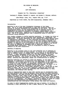
2.2 Example 1: a 5 GHz receiver front-end The approach of FAST is compared to ADS on the simulation of a 5 GHz WLAN receiver front-end (see Figure 1).

1

ADC

IF = 250 MHz

10-1

90O

LO1

Q

CPU time (normalized)

LO2 (250 MHz) ADC

MATLAB or ADS

MATLAB + MRMC

10-2

FAST

I 10-3

Figure 1: high-level simulation of the 5 GHz receiver front-end (left): if the special MRMC signal representation of FAST is used in MATLAB, then the CPU time drops with a factor 70. This is still ten times slower than with FAST itself, thanks to the scheduler of FAST that fully exploits the capabilities of the CPU. The CPU time with ADS is about the same as with MATLAB without the MRMC representation. The CPU time per timepoint for a FAST simulation of the complete receiver front-end of Figure 1 equals 9.78 µs on a Pentium II 266 MHz processor. The input at the antenna is an OFDM signal with 256 carriers, each with a QAM 16 modulation. The carrier frequency fc is 5.25 GHz. In addition to the input signal, two other waveform generators have been used for the two local oscillators (LO1 and LO2). These generators produce a sinusoidal signal with phase noise. Their frequency is fLO1 = 5 GHz and fLO2 = 0.25 GHz. The LNA is a static nonlinearity, described by a polynomial of order three that relates the output to the input. The coefficients of this polynomial are related to the intercept points [22]. The three mixers in this example are also described with a thirdorder polynomial, but now as a function of two inputs, the local oscillator input and the RF input. All filters in the front-end are elliptic filters. The RF bandpass filter has order three, the bandpass filter at 250 MHz order four, and the lowpass filters order six. Finally, the analog-to-digital converters (ADC) are ideal samplers that quantize the signal with a given resolution. A simulation of the receiver front-end of Figure 1 with FAST is ten times faster than with MATLAB where the MRMC signal representation of FAST is implemented. Without the use of this MRMC signal representation in MATLAB, FAST is 700 times more efficient than MATLAB. The latter does not introduce any approximation error due to integration methods, FFT leakage, digital filtering, … Therefore, its simulation results can be considered as the reference to check the accuracy of the other approaches. For the simulation of the receiver front-end of Figure 1, the error introduced with FAST (due to the use of digital filters) does not exceed –60 dB anywhere in the front-end. The same receiver front-end has been simulated with the envelope simulator of ADS [6, 9]. Hereby, two independent carriers have been chosen for the harmonic balance simulation, namely a carrier at fc = 5.25 GHz and a carrier at 250 MHz. This means that for each timestep we have a two-tone harmonic balance approach in which for each carriers three harmonics have been taken

into account. The different combinations of two tones are computed everywhere in the circuit, whereas FAST can discard frequencies at some places in the circuit where a frequency component is below a certain (user-definable) threshold. The input signal, which is the carrier at 5.25 GHz, is modulated in the same way as in the FAST and MATLAB simulations. The effects on the modulation are simulated in the time domain with a timestep that is equal to the inverse of the difference in frequency between two adjacent carriers. With this timestep ADS is about as slow as MATLAB without the MRMC representation. Furthermore, the results between ADS on one hand and FAST or MATLAB on the other hand, differ up to a few decibels. This is – at least partially – due to the approximations made by the numerical integration method [23]. These differences decrease when the timestep for the time-domain simulation part is increased. This of course requires more CPU time in ADS.

2.3 Example 2: a complete 5 GHz link Thanks to its dataflow nature, FAST can be coupled fairly easily with a digital simulator. In this way, FAST has been coupled with the digital modeling and simulation environment OCAPI [24], also developed at IMEC. As an example, a complete end-to-end simulation of a WLAN link (see Figure 2) taking into account a complete receiver front-end and a complete receiver modem is possible at a reasonable CPU time (0.35 seconds per OFDM symbol). DAC Tx Data

Modem Modem in in Tx Tx mode mode

Tx Data

Rx Data

OFDM OFDM Symbol Symbol Demapper Demapper

ADC Tx Tx Front-End Front-End

Channel Channel Model Model

OFDM OFDM Symbol Symbol Mapper Mapper

IFFT IFFT FFT FFT

Reference Reference Sequence Sequence

Guard Guard Removal Removal

Frequency Frequency Domain Domain Equalizer Equalizer

Rx Rx Front-End Front-End

Symbol Reordering

Modem Modem in in Tx Tx mode mode

Acquisition Sequence Guard Insertion

Time Time Domain Domain Synchronization Synchronization

Rx Data

DAC

ADC

MP-Interface MP-Interface Burst Burst Controller Controller

Microprocessor

Figure 2: a complete 5 GHz WLAN link that is simulated with the coupled FAST-OCAPI environment. The digital blocks are described at the dataflow level in fixed-point representation. The receiver front-end is the one from Figure 1. The CPU time is 0.35 s per OFDM symbol (96 bits) on a Pentium III 933 MHz with 512 MB RAM.

In the OCAPI environment the digital blocks can be represented at different abstraction levels, ranging from untimed descriptions (used in dataflow simulations) to timed descriptions (which can be specified down to the VHDL or Verilog level). The untimed representation is mostly used in architectural simulations. Hereby signals and constants (e.g. filter coefficients) can be represented as as a mix of fixed and floating-point numbers. The combination FAST-OCAPI offers the possibility to capture non-idealities of digital and analog blocks in one single simulation. Also, it allows to study digital compensation techniques for signal degradations that occur in the analog domain. For example, in a 5 GHz WLAN transceiver the multicarrier modulation gives rise to instantaneous large signal peaks. The large ratio between these peaks and the average signals necessitates the use of a large number of bits for the signals. In practice, the number of bits is limited such that some peaks are clipped to a saturation value. Despite the clipping in the transmit part of the digital modem, there are still large peaks that reach the power amplifier and drive this circuit into saturation. Some amount of nonlinear behavior in the power amplifier can be tolerated, since the equalizer in the digital part of the receiver can reconstruct the distorted signal to some extent. This is illustrated with the FAST-OCAPI simulation results of Figure 3. Mixed-signal compensation is not limited to forward correction. The coupled FAST-OCAPI simulator can be used to implement a feedback topology as well, for example modelling automatic gain control with digital steering of an analog variable gain amplifier.

2.4 Efficient bit-error-rate simulations The performance of a complete telecom link is often quantified with the biterror-rate (BER). This measure is typically determined with lengthy MonteCarlo simulations. In [25] a methodology is described that reduces the CPU time to determine the BER by more than two orders of magnitude, compared to Monte-Carlo simulations. This methodology is specific for telecom applications that use a multicarrier modulation scheme. Examples of such modulation are OFDM, used in 5 GHz WLAN, and ADSL. An OFDM-modulated signal consists of a sum of carriers, each being modulated using a separate modulation scheme such as Phase Shift Keying (PSK), Quadrature Amplitude Modulation (QAM), ... An OFDM symbol then gives rise to a specific constellation point in the modulation for each carrier. For some symbols, the different carriers can combine in a constructive way such that large peaks occur. The large signal peaks can lead to severe nonlinear distortion (e.g. saturation), which can increase the BER significantly. A practical measure to characterize an OFDM signal is the crest factor CF. This is the ratio of the maximum amplitude over the root-mean-square value of the signal. An efficient way for accurate BER estimations in multicarrier systems requires a dedicated approach. Indeed, measurement and/or simulation of the nonlinear effects on all possible symbols is not feasible. For example, an OFDM

modulation which uses 256 carriers and a 16-QAM modulation has 16256 possible symbols to transmit.

transmitted signal QPSK + BPSK pilots + zero carriers

10 dB back-off without equalization

0 dB back-off

with equalization

Figure 3: simulation result from FAST-OCAPI of the effect of an equalizer (5 GHz WLAN transceiver) on the constellation points that are distorted by several non-idealities. For this simulation, the nonlinearity of the power amplifier has been changed. With a 10 dB back-off, the equalizer manages to keep the BER low: there is a relative good correspondence between the constellation points of the input signal (figure at the top) and the constellation points at the output of the equalizer (bottom left). With a 0 dB back-off many constellation points are mapped erroneously (bottom right). A Monte-Carlo approach, on the other hand, would still require the generation of many symbols, since the ones that give rise to the high signal peaks, and hence to bit errors, have a fairly low probability of occurrence. To lower the required number of experiments to obtain a given accuracy on the BER, the method of [25] proceeds as follows: prior to simulation, a large number of OFDM symbols is generated. These are classified in sets according to their crest factor. For each set a BER is computed. These BER values together with the probability of occurrence of each crest factor value are combined to obtain the overall BER. This probability has been computed before the actual simulation. It only needs to be done once for a given modulation scheme. The BER for each set of symbols with the same crest factor is computed either with a Monte-Carlo method or with a quasi-analytical method. The latter approach which is used for low crest factors, considers the in-band distortion as Gaussian distributed noise.

This noise is computed based on simulation results and it is used in an analytical formula to compute the BER. For high crest factors, the assumption of having Gaussian distributed noise can be violated. Then a Monte-Carlo approach can be used with a higher accuracy but with a comparable efficiency. Indeed, the number of required experiments is low, since the probability of bit errors is high for large crest factors. Using this methodology, the BER of the WLAN link of Figure 2 is determined in one hour (Pentium II, 266 MHz) with the coupled FAST-OCAPI environment and with the models for the analog and digital blocks as in Figure 1 and 2. This is more than 100 times faster than with a pure Monte-Carlo approach for the same accuracy on the BER (see Figure 4).

2.5

x 10 -5 Monte Carlo Efficient method

2

BER

1.5

1

0.5 0 10 3

10 4

10 5

10 6

Number of Monte Carlo Experiments

Figure 4: computation of the BER of the WLAN link of Figure 2 with a Monte-Carlo approach and with the approach of [25]. The Monte-Carlo approach yields a higher accuracy on the BER when the number of experiments is increased, and it slowly converges to the final value. The approach of [25] obtains this final value in 3840 experiments, which is more than two orders of magnitude less experiments than with Monte-Carlo.

3 High-level models of analog blocks Analog circuits are inherently nonlinear. This complicates simulation. Moreover, it is much more difficult to construct a high-level model that takes into account nonlinear behavior than a linear model. One of the reasons is that electrical engineers have sufficient knowledge on linear system theory, but usually not on nonlinear systems. To overcome these difficulties, we have developed a methodology [26, 27] that can generate a high-level model from a given circuit (specified as a netlist) with only the dominant nonlinearities. Further, the methodology splits the nonlinear behavior of the total circuit into different contributions, one contribution for each nonlinearity. Since a

contribution consists of static nonlinearities and linear transfer functions, it can be interpreted. In this way, this methodology provides high-level models as well as insight into the nonlinear operation of a circuit. The approach yields models that take into account the frequency dependence of the nonlinear behavior of the circuit under consideration. The approach is limited to weakly nonlinear behavior. The weak nonlinearities of a circuit are described as power series that are broken down after the first few terms. For example, the drain current of a MOS transistor is described as a threedimensional power series of three variables, vGS, vDS and vSB. Each coefficient in this power series, referred to as a nonlinearity coefficient, can give rise to a contribution of the nonlinear behavior. As another example, the small-signal collector current ic as a function of the AC value vbe and the DC value VBE of the base-emitter voltage is given by

      VBE  v  ic = I S exp ⋅ exp be  kT  kT   q  q    

   ≈ g ⋅ v + K 2 v 2 + K 3gm v 3 + K m be gm be be   

(1)

where K2gm and K3gm are the second- and third-order nonlinearity coefficients, respectively. These are proportional to the second- and third-order derivatives of the transistor model equation. The modeling methodology has been implemented in a program called DISHARMONY. This program computes approximations of the Fourier transforms of Volterra kernels [22]. The first-order kernel transform describes the linear behavior of the circuit. The second-order and third-order kernel transforms, which are functions of two and three frequency variables, respectively, describe the second- and third-order nonlinear behavior. DISHARMONY first computes the exact values of the Fourier transforms. This is performed by combining AC analyses on the netlist of the circuit under consideration, together with a knowledge of nonlinearity coefficients, which are determined with DC circuit simulations. The Volterra kernel transforms that have been computed in this way contain many contributions, namely one for each second- or third-order coefficient of the power series description of the different nonlinearities in the circuit. Next, DISHARMONY determines the contributions that are dominant (up to a userdefinable error). A translation of the dominant contributions into a block diagram yields the final model. In most practical circuits usually few contributions dominate. This leads to compact high-levels that can be evaluated efficiently during high-level simulations. Moreover, a knowledge of the dominant contributions yields insight in the nonlinear circuit behavior. As an illustration, Figure 5 shows a 5 GHz low-noise amplifier and its high-level model generated by DISHARMONY. In this circuit transistor T3 is the amplifying transistor. The

rest of the circuit provides the necessary bias. It is found by DISHARMONY that the largest contribution to the second-order nonlinear behavior originates from the nonlinearity coefficient K2gm of the collector current power series expansion of T3. Other nonlinearities of T3, such as the base current, the nonlinear diffusion and junction capacitors and the base resistance, yield a negligible contribution. Also, the influence of the other transistors is negligible. For the third-order nonlinear behavior, the nonlinearity coefficients K2gm and K3gm of T3 yield the most important contributions. These three contributions suffice for an accurate high-level model. In addition to the generation of a high-level model, DISHARMONY also offers the possibility to interpret this model, since it consists of linear transfer functions, scale factors (namely the nonlinearity coefficients) and static nonlinearities (x2, x3 or an ideal multiplier). The transfer functions can be interpreted. For example, Ha(s) is the transfer function from the input to the base-emitter voltage of T3. The nonlinearity of the collector current of T3 produces from the signal at the base-emitter voltage a second-order and thirdorder nonlinear current. These currents correspond to the two last terms of equation (1). They propagate through the rest of the circuit (via transfer function Hc(s)) to form the second- and third-order output respectively of the circuit. Vcc R3

L T1

T2

R1

In R2

Out

T3

C

Ha (s)

input

Hb(s)

x2

+

K2gm3

Hd(s)

x3

+

output

Hc(s)

K3gm3

Figure 5: a 5 GHz BiCMOS low-noise amplifier and its high-level model, generated by DISHARMONY. The model only shows the nonlinear transfer from input to output. It can be completed with linear input and output impedances (that can also be frequency dependent). The result is a model that does not require iteration during simulation.

The models generated by DISHARMONY take into account the frequency dependence of the nonlinear behavior in a natural way. The need to take into account this frequency dependence is evident in wideband applications. In narrowband applications, the variation over the frequency band of interest can be neglected. In that case the transfer functions such as the ones shown in Figure 5, reduce to complex numbers. In this way, the model predicts the correct phase shift (e.g. expressed in terms of AM-PM conversion) of the nonlinear response. This is a more complete description than just an intercept point, which is a fixed real number (not a complex one) that does not model any phase shifts. Accurate high-level models used in FAST can be determined based on simulations, as is done with DISHARMONY, but also on measurements [28]. As an example, a high-level model for use in FAST has been derived for the 5 GHz low-noise amplifier of Figure 6, based on nonlinear S-parameter measurements. In this model the nonlinear dependencies are described as loworder nonlinear rational functions that do not require iterations during simulation.

Figure 6: a 5 GHz low-noise amplifier and its realization on a glass substrate. A model of this amplifier that has been determined based on measurements, takes into account the frequency dependence, the nonlinear behavior and the impedances at input and output. Evaluation of this model in FAST requires 0.12 µs per timestep (Pentium III processor).

4 Towards a mixed-signal design flow A modeling approach such as DISHARMONY and a high-level simulator such as FAST can only find acceptance in the design community if they can be linked in an elegant way to design tools at the circuit level and the layout level. A possible design flow that links the high level to the levels below is shown in Figure 7.

high-level models

architecture specs

(top-down or bottom-up)

high-level simulation

DISHARMONY

bottom-up modelling

FAST

specs for individual blocks circuit-level synthesis dimensions, bias values layout

silicon

Figure 7: a design flow for the analog front-end blocks that links the architectural level with the circuit and layout level. The design flow starts with a high-level simulation of a front-end architecture. At this stage analog-digital tradeoffs can be made. Afterwards, the architecture is split into analog and digital parts according the chosen tradeoff. The digital parts are designed in a separate design flow (not shown in Figure 7) [29]. During the first high-level simulations the models for the analog blocks are very rough. They could be generated by hand at this stage. From the high-level simulations an initial set of specifications for the individual analog/RF circuit blocks is derived. These serve as input for the circuit-level design. This can be performed in a manual way or using analog synthesis tools [30]. After the circuit design, the layout can be generated. Again, CAD tools for analog placement and routing could be used here to speed up the process [31]. The design flow as described up till now is a top-down process. The reliability of the results however very much depends on the high-level models used to model the behavior of the different blocks. The flow therefore also contains a bottom-up path in the form of verification using bottom-up models that are generated automatically from a circuit netlist. In this verification stage DISHARMONY can be used to extract a reliable high-level model that is consistent with the circuit that has been designed. These models are more accurate than the models that have been used initially, such that high-level simulations are now more reliable, leading to more realistic specifications for the analog circuits. Moreover, the accuracy of the DISHARMONY model is user-definable, such that the user can control the consistency between a circuit and the corresponding high-level model. This design flow splits the analog and the digital parts completely after the high-level tradeoffs have been made. This split neglects possible interference between the digital and the analog domain, as discussed in the next section.

5 Conclusions Modern telecom front-ends require intelligent tradeoffs between analog and digital to meet the stringent specifications. These tradeoffs are made at the architectural level and their effectiveness is tested with bit-error-rate (BER) simulations. This paper has shown several methodologies to efficiently perform this task: a high-level simulator FAST, a modeling methodology DISHARMONY that yields accurate high-level models for analog circuits, and an efficient BER estimation method for multicarrier modulation schemes such as WLAN. Per simulation step, FAST is more than two orders of magnitude faster than commercial approaches. In addition, the presented BER estimation method reduces the number of experiments with more than two orders of magnitude compared to a Monte-Carlo approach. This method, combined with FAST, can compute BER values of the order of 10-5 in CPU times of about one hour for a complete WLAN link with high-level models that take into account non-idealities in the analog and the digital domain. Together with an approach for high-level modeling of substrate noise caused by digital circuits, these tools can be integrated in a mixed-signal flow for the design of advanced architectures of front-ends of wireless terminals.

6 References [1] SABER of Avant!, http://www.avanticorp.com/ [2] Jeruchim, Balaban and Shanmugan, "Simulation of Communication Systems," Plenum, 1992. [3] F. Medeiro, B. Perez-Verdu, A. Rodriguez-Vazquez and J.L. Huertas, “A vertically integrated tool for automated design of Σ∆ modulators,” IEEE J. Solid-State Circuits, vol. 30, no. 7, pp. 762-772, July 1995. [4] J. Vandenbussche, G. Van der Plas, G. Gielen and W. Sansen, “Behavioral model of reusable D/A converters,” IEEE Trans. Circuits and Systems II: Analog and digital signal processing, vol. 46, no. 10, pp. 1323-1326, Oct. 1999. [5] A. Abidi, “Behavioral modeling of analog and mixed signal IC’s,” Proc. Custom Integrated Circuits Conference, pp. 443-450, May 2001. [6] J.L. Pino and K. Kalbasi, “Cosimulating synchronous DSP applications with analog RF circuits,” Proc. 32nd Annual Asilomar Conference on Signals, Systems, and Computers, Nov. 1998. [7] E. Ngoya and R. Larchevèque, “Envelop transient analysis: a new method for the transient and steady state analysis of microwave communication circuits and systems,” Proc. IEEE MTT-S, pp. 1365-1368, 1996. [8] K. Kundert, J. White and A. Sangiovanni-Vincentelli, “An envelopefollowing method for the efficient transient simulation of switching power and filter circuits,” Proc. IEEE International Conference on ComputerAided Design, November 1988. [9] HP-ADS of Hewlett-Packard, http://www.tm.agilent.com/tmo/hpeesof/products/ads/adsoview.html. [10] SPW of Cadence, http://www.cadence.com/products/spw.html

[11] COSSAP of Synopsys, http://www.synopsis.com/products/dsp/cossap_ds.html . [12] Gerd Vandersteen, Piet Wambacq, Yves Rolain, Petr Dobrovolný, Stéphane Donnay, Marc Engels, Ivo Bolsens, “A methodology for efficient high-level dataflow simulation of mixed-signal front-ends of digital telecom transceivers”, Proc. Design Automation Conference, pp.440-445, 2000. [13] I. Vassiliou and A. Sangiovanni-Vincentelli, “A frequency-domain, Volterra series-based behavioral simulation tool for RF systems,” Proc. IEEE Custom Integrated Circuits Conference, pp. 21-24, 1999. [14] P. Vanassche, G. Gielen, “Efficient Time-Domain Simulation of Telecom Frontends Using a Complex Damped Exponential Signal Model”, Proc. DATE 2001. [15] SubstrateStorm of Simplex, http://www.simplex.com. [16] M. van Heijningen, M. Badaroglu, S. Donnay, M. Engels and I. Bolsens, “High-Level Simulation of Substrate Noise Generation Including Power Supply Noise Coupling”, Proc. Design Automation Conference, pp. 446451, 2000. [17] M. van Heijningen, J. Compiet, P.Wambacq, S. Donnay M. Engels and I. Bolsens, “Modeling of Digital Substrate Noise Generation and Experimental Verification Using a Novel Substrate Noise Sensor”, IEEE Journal of Solid-State Circuits, vol.35, pp.1002-1008, July 2000. [18] M. van Heijningen, M. Badaroglu, S. Donnay, H. De Man, G. Gielen, M. Engels and I. Bolsens, “Substrate noise generation in complex digital systems: efficient modeling and simulation methodology and experimental verification”, Proc. International Solid-State Circuit Conference, pp. 342343, 2001. [19] M. Badaroglu, M. van Heijningen, V. Gravot, J. Compiet, S. Donnay, M. Engels, G. Gielen and H. De Man, “Methodology and Experimental Verification for Substrate Noise Reduction in CMOS Mixed-Signal ICs with Synchronous Digital Circuits”, Proc. IEEE International Solid-State Circuits Conference, 2002. [20] K. Kundert, J. White and A. Sangiovanni-Vincentelli, “Steady-state methods for simulating analog and microwave circuits,” Kluwer Academic Publishers, 1990. [21] J. Chen, D. Feng, J. Philips and K. Kundert, “Simulation and modeling of intermodulation distortion in communication circuits,” Proc. IEEE Custom Integrated Circuits Conference, pp. 5-8, 1999. [22] P. Wambacq and W. Sansen, “Distortion analysis of analog integrated circuits,” Kluwer Academic Publishers, 1998. [23] K. Kundert and P. Gray, “The designer’s guide to SPICE and Spectre,” Kluwer Academic Publishers, 1995. [24] P. Schaumont et al., "A programming environment for the design of complex high speed ASICs", Proc. Design Automation Conference, pp. 315-320, June 1998.

[25] Gerd Vandersteen, Piet Wambacq, Yves Rolain, Johan Schoukens, Stéphane Donnay, Marc Engels and Ivo Bolsens, “Efficient Bit-Error-Rate estimation of multicarrier transceivers,” Proc. DATE 2001. [26] P. Wambacq, P. Dobrovolný, S. Donnay, M. Engels and I. Bolsens, “Compact modeling of nonlinear distortion in analog communication circuits”, Proc. DATE 2000. [27] P. Dobrovolny, P. Wambacq, G. Vandersteen, S. Donnay, M. Engels and I. Bolsens, “Bottom-up generation of accurate complex lowpass equivalent of integrated RF ICs for 5 GHz WLAN”, Proc. IEEE MTT-S International Microwave Symposium, Vol. 1, pp. 419-22, Phoenix (AZ), USA, May 2001. [28] G. Vandersteen, F. Verbeyst, P. Wambacq and S. Donnay, “Highfrequency nonlinear amplifier model for the efficient evaluation of inband distortion under nonlinear load-pull conditions”, Proc. DATE 2002. [29] D. Verkest, W. Eberle, P. Schaumont, B. Gyselinckx and S. Vernalde, “C++ based system design of a 72 Mb/s OFDM transceiver for WLAN,” Proc. Custom Integrated Circuits Conference, pp. 433-439, 2001. [30] G. Van der Plas et al., “AMGIE – a synthesis environment for CMOS analog integrated circuits,” IEEE Trans. On Computer-Aided Design, vol. 20, no. 9, pp. 1037-1058, September 2001. [31] K. Lampaert, G. Gielen and W. Sansen, Analog layout generation for performance and manufacturability, Kluwer Academic Publishers, Dordrecht, the Netherlands, 1999.