High-Level Why-Not Explanations using Ontologies [New Formal Framework Paper]
Balder ten Cate LogicBlox and UCSC
Cristina Civili Sapienza Univ. of Rome
Evgeny Sherkhonov Univ. of Amsterdam
Wang-Chiew Tan UCSC
arXiv:1412.2332v1 [cs.DB] 7 Dec 2014
{
[email protected],
[email protected],
[email protected],
[email protected] }
ABSTRACT
1. INTRODUCTION AND RESULTS
We propose a novel foundational framework for why-not explanations, that is, explanations for why a tuple is missing from a query result. Our why-not explanations leverage concepts from an ontology to provide high-level and meaningful reasons for why a tuple is missing from the result of a query. A key algorithmic problem in our framework is that of computing a most-general explanation for a why-not question, relative to an ontology, which can either be provided by the user, or it may be automatically derived from the data and/or schema. We study the complexity of this problem and associated problems, and present concrete algorithms for computing why-not explanations. In the case where an external ontology is provided, we first show that the problem of deciding the existence of an explanation to a why-not question is NP-complete in general. However, the problem is solvable in polynomial time for queries of bounded arity, provided that the ontology is specified in a suitable language, such as a member of the DL-Lite family of description logics, which allows for efficient concept subsumption checking. Furthermore, we show that a most-general explanation can be computed in polynomial time in this case. In addition, we propose a method for deriving a suitable (virtual) ontology from a database and/or a data workspace schema, and we present an algorithm for computing a most-general explanation to a why-not question, relative to such ontologies. This algorithm runs in polynomial-time in the case when concepts are defined in a selection-free language, or if the underlying schema is fixed. Finally, we also study the problem of computing short mostgeneral explanations, and we briefly discuss alternative definitions of what it means to be an explanation, and to be most general.
An increasing number of databases are derived, extracted, or curated from disparate data sources. Consequently, it becomes more and more important to provide data consumers with mechanisms that will allow them to gain an understanding of data that they are confronted with. An essential functionality towards this goal is the capability to provide meaningful explanations about why data is present or missing from a database. There has been considerable research on this general topic. In particular, there is a body of work on deriving explanations for why a tuple belongs to the output of a query, and also why a tuple is missing from the output of a query. Systems were developed in [2, 25] to provide explanations for answers to logic programs in the context of a deductive database. The presence of a tuple in the output is explained by enumerating all possible derivations, that is, instantiations of the logic rules that derive the answer tuple. In [25], the system also explains missing answers, by providing a partially instantiated rule, based on the missing tuple, and leaving the user to figure out how the rest of the rule would have to be instantiated. In the last decade or so, there has been significant efforts to characterize different notions of provenance (or lineage) of query answers (see, e.g., [13, 16]) which can also be applied to understand why an answer is in the query result. By comparison, there has been less work on the why-not problem, that is, the problem of explaining why an answer is missing from the output. Since [25], the why-not problem was also studied in [18, 19] in the context of “debugging” results of data extracted via select-project-join queries, and, subsequently, a larger class of queries that also includes union and aggregation operators. Unlike [25] which is geared towards providing explanations for answers and missing answers, the goal in [19] is to propose modifications to underlying database I, yielding another database I ′ based on the provenance of the missing tuple, constraints, and trust specification at hand, so that the missing tuple appears in the result of the same query q over the updated database I ′ . In contrast to the data-centric approach of updating the database to derive the missing answer, another line of research [5, 12, 26] follows a query-centric approach whereby the query q at hand is modified to q ′ (without modifying the underlying database) so that the missing answer appears in the output of q ′ (I). In this paper, we develop a novel foundational framework for why-not explanations that is principally different from prior approaches. Our approach is neither data-centric nor query-centric. Instead, we derive high-level explanations via an ontology that is either provided, or is derived from the data or schema. Our immediate goal is not to repair the underlying database or query so that the missing answer would appear in the result. Rather, as in [25], our goal is to provide explanations for why an answer is missing
Categories and Subject Descriptors H.2 [Database Management]
General Terms Theory, Algorithms
Keywords Databases, Why-Not Explanations, Provenance, Ontologies
Permission to make digital or hard copies of all or part of this work for personal or classroom use is granted without fee provided that copies are not made or distributed for profit or commercial advantage and that copies bear this notice and the full citation on the first page. To copy otherwise, to republish, to post on servers or to redistribute to lists, requires prior specific permission and/or a fee. PODS ’15 Melbourne, Australia Copyright 20XX ACM X-XXXXX-XX-X/XX/XX ...$15.00.
from the query result. As we will illustrate, explanations that are based on an ontology have the potential to be high-level and provide meaningful insight to why a tuple is missing from the result. Formally, an explanation for why a tuple a is not among the results of a query q(I), in our framework, is a tuple of concepts from the ontology whose extension includes the missing tuple a and, at the same time, does not include any tuples from q(I). For example, a query may ask for all products that each store has in stock, in the form of (product ID, store ID) pairs, from the database of a large retail company. A user may then ask why is the pair (P0034, S012) not among the result of the query. Suppose P0034 refers to a bluetooth headset product and S012 refers to a particular store in San Francisco. If P0034 is an instance of a concept bluetooth headsets and S012 is an instance of a concept stores in San Francisco, and suppose that no pair (x, y), where x is an instance of bluetooth headset and y is an instance of stores in San Francisco, belongs to the query result. Then the pair of concepts (bluetooth headset, stores in San Francisco) is an explanation for the given why-not question. Intuitively, it signifies the fact that “none of the stores in San Francisco has any bluetooth headsets on stock”. There may be multiple explanations for a given why-not question. In the above example, this would be the case if, for instance, S012 belongs also to a more general concept stores in California, and that none of the stores in California have bluetooth headsets on stock. Our goal is to compute a most-general explanation, that is, an explanation that is not strictly subsumed by any other explanation. We study the complexity of computing a most-general explanation to a why-not question. Formally, we define a why-not instance (or, why-not question) to be a quintuple (W, I, q, Ans, a) where W is a data workspace schema consisting of a data schema, a collection of view definitions (specified by means of a Datalog program over the data schema), and a set of integrity constraints; I is an instance of W consisting of the source and the materialized view relations; q is a query over W; Ans = q(I); and a 6∈ q(I). We note that why-not questions easily arise when querying data workspaces, especially when there is a large collection of views and where a view may be defined in terms of other views. Our motivation to investigate why-not questions also arises from practical concerns in application development at LogicBlox. In fact, data workspace schemas capture the core of LogiQL [17], the declarative data analytics language developed and used at LogicBlox [15]. Our framework supports a very general notion of an ontology, which we call S-ontologies. For a given relational schema S, an Sontology is a triple (C, ⊑, ext) which defines the set of concepts, the subsumption relationship between concepts, and respectively, the extension of each concept w.r.t. an instance of the schema S. We use this general notion of an S-ontology to formalize the key notions of explanations and most-general explanations, and we show that S-ontologies capture two different types of ontologies. The first type of ontologies we consider are those that are defined externally, provided that there is a way to associate the concepts in the externally defined ontology to the instance at hand. For example, the ontology may be represented in the form of a OntologyBased Data Access (OBDA) specification [23]. More precisely, an OBDA specification consists of a set of concepts and subsumption relation specified by means of a description logic terminology, and a set of mapping assertions that relates the concepts to a relational database schema at hand (in our case, the data workspace schema). Every OBDA specification induces a corresponding S-ontology. If the concepts and subsumption relation are defined by a TBox in a tractable description logic such as DL-LiteR, and the mapping assertions are Global-As-View (GAV) assertions, the induced Sontology can in fact be computed from the OBDA specification in
polynomial time. We then present an algorithm for computing all most-general explanations to a why-not question, given an external S-ontology. The algorithm runs in polynomial time when the arity of the query is bounded, and it executes in exponential time in general. We show that the exponential running time is unavoidable because the problem of deciding whether or not there exists an explanation to a why-not question given an external S-ontology is NP-complete in general. The second type of ontologies that we consider are ontologies that are derived either (a) from a data workspace schema W, or (b) from an instance of the data workspace schema. In both cases, the concepts of the ontology are defined through concept expressions in a suitable language LW that we develop. Specifically, our concepts are obtained from the relations in the schema, through selections, projections, and intersection. The difference between the two cases lies in the way the subsumption relation ⊑ is defined. In the former, a concept C is considered to be subsumed in another concept C ′ if the extension of C is contained in the extension of C ′ over all instances of the data workspace schema. For the latter, subsumption is considered to hold if the extension of C is contained in the extension of C ′ with respect to the given instance of the data workspace schema. The S-ontology induced by a data workspace schema W, or instance I, denoted OW or OI , respectively, is typically infinite, and is not intended to be materialized. Instead, we present an algorithm for directly computing a most-general explanation with respect to OI . The algorithm runs in exponential time in general. However, if the concepts are defined in the selection-free fragment of our concept language, or if the data workspace schema is fixed, it runs in polynomial time. As for computing most-general explanations with respect to OW , we identify restrictions on the datalog program and the integrity constraints under which the problem is decidable, and we present complexity upper bounds for these cases. More related work: The use of ontologies to facilitate access to databases is not new. A prominent example is OBDA, where queries are either posed directly against an ontology, or an ontology is used to enrich a data schema against which queries are posed with additional relations (namely, the concepts from the ontology) [6, 23]. Answers are computed based on an open-world assumption and using the mapping assertions and ontology provided by the OBDA specification. As we described above, we make use of OBDA specifications as a means to specify an external ontology and with a database instance through mapping assertions. However, unlike in OBDA, we consider queries posed against a database instance under the traditional closed-world semantics, and the ontology is used only to derive why-not explanations. The problems of providing why explanations and why-not explanations have also been investigated in the context of query ontologies in [8] and [10], respectively. The why-not explanations of [10] follow the data-centric approach to why-not provenance as we discussed earlier where their goal is to modify the assertions that describe the extensions of concepts in the ontology so that the missing tuple will appear in the query result. There has also been prior work on extracting ontologies from data. For example, in [20], the authors considered heuristics to automatically generate an ontology from a relational database by defining project-join queries over the data. Other examples on ontology extraction from data include publishing relational data as RDF graphs or statements (e.g., D2RQ [7], Triplify [3]). We emphasize that our goal is not to extract and materialize ontologies, but rather, to use an ontology that is derived from data to compute why-not explanations. Outline: After the preliminaries, in Section 3 we present our framework for why-not explanations. In Section 4 we discuss in
detail the two ways of obtaining an S-ontology. In Section 5 we present our main algorithmic results. Finally, in Section 6, we study variatations of our framework, including the problem of producing short most-general explanations, and alternative notions of explanation, and of what it means to be most general.
2.
PRELIMINARIES
A relational schema S is a set {R1 , . . . , Rn } of relation names, where each Ri has an associated arity. A fact is an expression of the form R(b1 , . . . , bk ) where R ∈ S is a relation of arity k, and for 1 ≤ i ≤ k, we have bi ∈ Const, where Const is a countably infinite set of constants. We assume a dense linear order < on Const. An attribute A of an k-ary relation name R ∈ S is a number i such that 1 ≤ i ≤ k. For a fact R(b) where b = b1 , . . . , bk , we sometimes write πA1 ,...,Ak (b) to mean the tuple consisting of the A1 th, ..., Ak th constants in the tuple b, that is, the value (bA1 , ..., bAk ). A database instance, or simply an instance, I over S is a set of facts over S. Equivalently, an instance I is a map that assigns to each k-ary relation name R ∈ S a finite set of k-tuples over Const. By RI we denote the set of these tuples. We write Inst(S) to denote the set of all database instances over S, and adom(I) to denote the active domain of I, i.e., the set of all constants occurring in facts of I. Queries A conjunctive query (CQ) over S is a query of the form q(x) :- Φ(x, y) where Φ(x, y) is a conjunction of atoms over S, and where q 6∈ S. The formula Φ(x, y) is called the body of the query while the atom q(x) is the head. Each variable in x is required to occur in the body. A boolean conjunctive query (BCQ) is a CQ whose head relation q has zero arity. A conjunctive query with comparisons is a a conjunctive query where the body may, in addition, contain expressions of the form x op c, where op ∈ {=, , ≤, ≥} and c ∈ Const. Given an instance I and a CQ q with or without comparisons, we write q(I) to denote the set of answers of q over I. A Datalog program Π is a set of rules where each rule has the form α(x) :- Φ(x, y). As in the above definition of conjunctive queries, α(x) (the head of the rule) is an atom with α 6∈ S and Φ(x, y) (the body of the rule) is a conjunction of atoms and expressions of the form x op c, where op ∈ {=, , ≤, ≥} and c ∈ Const. Each variable in x is required to occur in the body. Unlike CQs, however, the same relation can occur in both the head and body of the same rule. The fact that we allow comparisons with constants in the Datalog program has no impact on our complexity results. That is, all results stated in the paper apply also in the case where Datalog programs are not allowed to contain comparisons with constants. The relations occurring in Π are classified as extensional database relations (EDBs), if they do not occur in the head of any rule, or intensional database relations (IDBs) otherwise. The EDBs and IDBs of a Datalog program Π are denoted by EDB(Π) and IDB(Π), respectively. A Datalog query is a Datalog program with a distinguished IDB G, which is called the goal relation. We distinguish between different types of Datalog programs. A relation P immediately depends on another relation P ′ if there is a rule in Π that has P in the head and P ′ in the body. A Datalog program is non-recursive if the depends relation is acyclic. A Datalog program is linear if, for every rule, the body of the rule contains at most one occurrence of an IDB. A Datalog program is said to be a collection of UCQ-view definitions if, for every rule, the body of the rule contains no IDB relations and no comparisons. Note that a collection of UCQ-view definitions is a special case of a linear
non-recursive Datalog program. For a Datalog program Π and an instance I of the schema EDB(Π), by Π(I) we denote the least fixed point of I with respect to to Π, that is, the (unique) smallest instance J over the schema IDB(Π) such that (I, J) satisfies the rules of Π. Integrity constraints We consider two common classes of integrity constraints: functional dependencies and inclusion dependencies. A functional dependency (FD) on a relation R ∈ S is an expression of the form R : X → Y where X and Y are subsets of the set of attributes of R. We say that an instance I over S satisfies the FD if for every a1 and a2 from RI if πA (a1 ) = πA (a2 ) for every A ∈ X, then πB (a1 ) = πB (a2 ) for every B ∈ Y . An inclusion dependency (ID) is an expression of the form R[A1 , . . . , An ] ⊆ S[B1 , . . . , Bn ] where R, S ∈ S, each Ai and Bj is an attribute of R and S respectively. We say that an instance I over S satisfies the ID if {πA1 ,...,An (a) | a ∈ RI } ⊆ {πB1 ,...,Bn (b) | b ∈ S I }. Data Workspaces We are interested in the scenario where we have a database instance I that conforms to a relational schema (called the data schema) D, a Datalog program Π that defines a collection V of materialized views over D, and a set Σ of integrity constraints over D∪IDB(Π). We formalize this scenario through the concept of a data workspace schema. A data workspace schema is a quadruple (D, V, Π, Σ) where D and V are disjoint relational schemas (whose elements are called base relations and view relations, respectively); Π is a Datalog program whose IDBs are the relations in V and whose EDBs belong to D; and Σ is a collection of integrity constraints over D ∪ V. An instance of a data workspace schema W is a relational database instance I over the schema D ∪ V such that Π(ID ) = IV and I |= Σ, where ID and IV denote the restriction of I to relations in D and V, respectively. Intuitively, a data workspace schema defines the relations that one may work with, whether they are base relations or materialized view relations. By a query over W, we mean a query that is posed over D ∪ V. Simple relational database schemas without views or constraints are a special case of data workspace schemas, where V, Π, and Σ are empty. Example 2.1. As an example data workspace schema, consider W = (D, V, Π, Σ), where each element of the quadruple is shown in Figure 1. An instance I = ID ∪ IV of the data workspace schema W is given in Figure 2. ✷
3. WHY-NOT EXPLANATIONS Next, we introduce our ontology-based framework for explaining why a tuple is not in the output of a query. Our framework is based on a general notion of an ontology. As we shall describe in Section 4, the ontology that is used may be an external ontology (for example, an existing ontology specified in a description logic), or it may be an ontology that is derived from a data workspace. Both are a special case of our general definition of an S-ontology. Definition 3.1 (S-ontology). An S-ontology over a relational schema S is a triple O = (C, ⊑, ext), where • C is a possibly infinite set, whose elements are called concepts, • ⊑ is a pre-order (i.e., a reflexive and transitive binary relation) on C, called the subsumption relation, and
ID
Data schema D : {Cities(name, population, country, continent), Train-Connections(city_from, city_to)} View schema V : {BigCity(name), EuropeanCountry(name), Reachable(city_from, city_to)} Datalog Program Π: BigCity(x) EuropeanCountry(z) Reachable(x,y) Reachable(x,y)
:– :– :– :–
Cities(x,y,z,w), y ≥ 5000000 Cities(x,y,z,w), w = Europe Train-Connections(x,y) Train-Connections(x,z), Train-Connections (z,y)
Integrity constraints Σ: country BigCity[name] Train-Connections[city_from] Train-Connections[city_to]
→ ⊆ ⊆ ⊆
continent Train-Connections[city_from] Cities[name] Cities[name]
Cities
Train-Connections
name Amsterdam Berlin Rome New York San Francisco Santa Cruz Tokyo Kyoto
population 779,808 3,502,000 2,753,000 8,337,000 837,442 59,946 13,185, 000 1,400,000
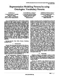
An example of an S-ontology O = (C, ⊑, ext) is shown in Figure 3, where the concept subsumption relation ⊑ is depicted by means of a Hasse diagram. Note that, in this example, ext(C, I) is independent of the database instance I (and, as a consequence, every S-instance is consistent with O). In general, this is not the case (for example, the extension of a concept may be determined through mapping assertions, cf. Section 4.1). We define our notion of an ontology-based explanation next. Definition 3.2 (Explanation). Let O = (C, ⊑, ext) be an Sontology, I an S-instance, q be an m-ary query over S, and a = (a1 , . . . , am ) a tuple of constants such that a 6∈ q(I). Then a tuple of concepts (C1 , . . . , Cm ) from C m is called an explanation for a 6∈ q(I) with respect to O (or an explanation in short) if: • for every 1 ≤ i ≤ m, ai ∈ ext(Ci , I), and • (ext(C1 , I) × . . . × ext(Cm , I)) ∩ q(I) = ∅. In other words, an explanation is a tuple of concepts whose extension includes the missing tuple a (and thus explains a) but, at the same time, it does not include any tuple in q(I) (and thus does not explain any tuple in q(I)). Intuitively, the tuple of concepts is an explanation that is orthogonal to existing tuples in q(I) but relevant for the missing tuple a, and thus forms an explanation for why a is not in q(I). There can be multiple explanations in general and the “best” explanations are the ones that are the most general. Definition 3.3 (Most-general explanation). Let O = (C, ⊑, ext) be an S-ontology, and let E = (C1 , . . . , Cm ) and E ′ = ′ (C1′ , . . . , Cm ) be two tuples of concepts from C m . • We say that E is less general than E ′ with respect to O, denoted as E ≤O E ′ , if Ci ⊑ Ci′ for every i, 1 ≤ i ≤ m. • We say that E is strictly less general than E ′ with respect to O, denoted as E O E. Example 3.1. Consider the instance ID of the relational schema S = {Cities(name, population, country, continent), TrainConnections(city_from, city_to)} shown in Figure 2. Suppose q is the query (x, y) :- Train-Connections(x, z), Train-Connections(z, y). That is, the query asks for all pairs of cities that are connected via a city. Then q(I) returns tuples {hAmsterdam, Romei, hAmsterdam, Amsterdami, hBerlin, Berlini, hNew York, Santa Cruzi}. A user may ask why is the tuple hAmsterdam, New Yorki not in the result of q(I) (i.e., why is hAmsterdam, New Yorki 6∈ q(I)?). Based on the S-ontology defined in Figure 3, we can derive the following explanations for hAmsterdam, New Yorki ∈ / q(I) : E1 E2 E3 E4
= = = =
hDutch-City, East-Coast-Cityi hDutch-City, US-Cityi hEuropean-City, East-Coast-Cityi hEuropean-City, US-Cityi
E1 is the simplest explanation, i.e., the one we can build by looking at the lower level of the hierarchy in our S-ontology. Each subsequent explanation is more general than at least one of the prior explanations w.r.t. to the S-ontology. In particular, we have E4 >O E2 >O E1 , and E4 >O E3 >O E1 . Thus, the mostgeneral explanation for why hAmsterdam, New Yorki 6∈ q(I) with respect to our S-ontology is E4 , which intuitively informs that the reason is because Amsterdam is a city in Europe while New York is a city in the US (and hence, they are not connected by train). Note that all the other possible combinations of concepts are not explanations because they intersect with q(I). ✷ As we will see in Example 4.3, there may be more than one mostgeneral explanations in general. Generalizing the above example, we can informally define the problem of explaining why-not questions via ontologies as follows: given an instance I of schema S, a query q over S, an S-ontology O, and a tuple a 6∈ q(I), compute a most-general explanation for
City
European-City
US-City
Dutch-City
East-Coast-City West-Coast-City
ext(City, I)
=
ext(European-City, I) ext(Dutch-City, I) ext(US-City, I) ext(East-Coast-City, I) ext(West-Coast-City, I)
= = = = =
{Amsterdam, Berlin, Rome, New York, San Francisco, Santa Cruz, Tokyo, Kyoto} {Amsterdam, Berlin, Rome} {Amsterdam} {New York, San Francisco, Santa Cruz} {New York} {Santa Cruz, San Francisco}
Figure 3: Example ontology. a 6∈ q(I), if one exists, w.r.t. O. The S-ontology O may be given explicitly as part of the input, or it may be derived from a given database instance or a given data workspace.
DL-Lite TBox axiom
(first-order translation)
EU-City ⊑ City Dutch-City ⊑ EU-City N.A.-City ⊑ City EU-City ⊑ ¬ N.A.-City US-City ⊑ N.A.-City City ⊑ ∃ hasCountry Country ⊑ ∃ hasContinent ∃hasCountry− ⊑ Country ∃hasContinent− ⊑ Continent ∃connected ⊑ City ∃connected− ⊑ City
∀x EU-City(x) → City(x) ∀x Dutch-City(x) → EU-City(x) ∀x N.A.-City(x) → City(x) ∀x EU-City(x) → ¬N.A.-City(x) ∀x US-City(x) → N.A.-City(x) ∀x City(x) → ∃y hasCountry(x, y) ∀x Country(x) → ∃y hasContinent(x, y) ∀x (∃y hasCountry(y, x)) → Country(x) ∀x (∃y hasContinent(y, x)) → Continent(x) ∀x (∃y connected(x, y)) → City(x) ∀x (∃y connected(y, x)) → City(x)
GAV mapping assertions (universal quantifiers omitted for readability): Cities(x, z, w, “Europe”) Cities(x, z, “Netherlands”, w) Cities(x, z, w, “N.America”) Cities(x, z, “USA”, w) Cities(x, y, z, w) Cities(x, k, y, w) Cities(x, k, w, y) Train-Connection(x, y), Cities(x, x1 , x2 , x3 ), Cities(y, y1 , y2 , y3 )
→ → → → → → →
EU-City(x) Dutch-City(x) N.A.-City(x) US-City(x) Continent(w) hasCountry(x,y) hasContinent(x,y)
→
connected(x,y)
Figure 4: Example DL-Lite ontology with mapping assertions.
4.
OBTAINING ONTOLOGIES
In this section we discuss two approaches by which S-ontologies may be obtained. The first approach allows one to leverage an external ontology, provided that there is a way to relate a concept in the ontology to a database instance. In this case, the set C of concepts is specified through a description logic such as ALC or DLLite; ⊑ is a partial order on the concepts defined in the ontology, and the function ext may be given through mapping assertions. The second approach is to consider an S-ontology that is derived from a specific database instance, or from a data workspace schema. In either case, we study the complexity of deriving such S-ontologies based on the language on which concepts are defined, the subsumption between concepts, and the function ext, which is defined according to the semantics of the concept language.
4.1 Leveraging an external ontology We first consider the case where we are given an external ontology that models the domain of the database instance, and a relationship between the ontology and the instance. We will illustrate in particular how description logic ontologies are captured as a special case of our framework. In what follows, our exposition borrows notions from the Ontology-Based Data Access (OBDA) framework. Specifically, we will make crucial use of the notion of an OBDA specification [14], which consists of a description logic ontology, a relational schema, and a collection of mapping assertions. To keep the exposition simple, we restrict our discussion to one particular description logic, called DL-LiteR , which is a representative member of the DL-Lite family of description logics [9]. DL-LiteR is the basis for the OWL 2 QL1 profile of OWL 2, which is a standard ontology language for Semantic Web adopted by W3C. As the other languages in the DL-Lite family, DL-LiteR exhibits a good trade off between expressivity and complexity bounds for important reasoning tasks such as subsumption checking, instance checking and query answering. TBox and Mapping Assertions. In the description logic literature, an ontology is typically formalized as a TBox (Terminology Box), which consists of finitely many TBox axioms, where each TBox axiom expresses a relationship between concepts. Alongside TBoxes, ABoxes (Assertion Boxes) are sometimes used to describe 1
http://www.w3.org/TR/owl2-profiles/#OWL_2_QL
the extension of concepts. To simplify the presentation, we do not consider ABoxes here. Definition 4.1 (DL-LiteR ). Fix a finite set ΦC of “atomic concepts” and a finite set ΦR of “atomic roles”. • The concept expressions and role expressions of DL-LiteR are defined as follows: Basic concept expression: Basic role expression: Concept expressions: Role expressions
B ::= A | ∃R R ::= P | P − C ::= B | ¬B E ::= R | ¬R
where A ∈ ΦC and P ∈ ΦR . Formally, a (ΦC , ΦR )interpretation I is a map that assigns to every atomic concept in ΦC a unary relation over Const and to every atomic role in ΦR a binary relation over Const. The map I naturally extends to arbitrary concept expressions and role expressions: I(P − ) = {(x, y) | (y, x) ∈ I(P )} I(¬P ) = Const2 \ I(P )
I(∃P ) = π1 (I(P )) I(¬A) = Const \ I(A)
Observe that I(∃P − ) = π2 (I(P )). • A TBox (Terminology Box) is a finite set of TBox axioms where each TBox axiom is an inclusion assertion of the form B ⊑ C or R ⊑ E, where B is a basic concept expression, C is a concept expression, R is a basic role expression and E is a role expression. An (ΦC , ΦR )-interpretation I satisfies a TBox if for each axiom X ⊑ Y , it holds I(X) ⊆ I(Y ). • For concept expressions C1 , C2 and a TBox T , we say that C1 is subsumed by C2 relative to T (notation: T |= C1 ⊑ C2 ) if, for all interpretations I satisfying T , we have that I(C1 ) ⊆ I(C2 ). An example of a DL-LiteR TBox is given at the top of Figure 4. For convenience, we have listed next to each TBox axiom, its equivalent semantics in first-order notation. Next we describe what mapping assertions are. Given an ontology and a relational schema, we can specify mapping assertions to relate the ontology language to the relational schema, which is similar to how mappings are used in OBDA [23]. In general, mapping
assertions are first order sentences over the schema S ∪ ΦC ∪ ΦR that express relationships between the symbols in S and those in ΦC and ΦR . Among the different schema mapping languages that can be used, we restrict our attention, for simplicity, to the class of Global-As-View (GAV) mapping assertions (GAV mapping assertions or GAV constraints or GAV source-to-target tgds). Definition 4.2 (GAV mapping assertions). A GAV mapping assertion over (S, (ΦC ∪ ΦR )) is a first-order formula of the form ∀~x (ϕ1 (~x), · · · , ϕn (~x)) → ψ(~x) where ϕ1 , . . . , ϕn are atomic formulas using relations from S and ψ is an atomic formula of the form A(xi ) (for A ∈ ΦC ) or P (xi , xj ) (for P ∈ ΦR ). Intuitively, a GAV mapping assertion associates a conjunctive query over S to an element (concept or atomic role) of the ontology. A set of GAV mapping assertions associates, in general, a union of conjunctive queries to an element of the ontology. Examples of GAV mapping assertions are given at the bottom of Figure 4. OBDA induced ontologies Definition 4.3 (OBDA specification). Let T be a TBox, S a relational schema, and M a set of mapping assertions from S to the concepts of T . We call the triple B = (T , S, M) an OBDA specification. An (ΦC , ΦR )-interpretation I is said to be a solution for an Sinstance I with respect to the OBDA specification B if the pair (I, I) satisfies all mapping assertions in M and I satisfies T . Note that our notion of an OBDA specification is a special case of the one given in [14], where we do not consider view inclusion dependencies. Also, as mentioned earlier, our OBDA specifications in this paper assume that T is a DL-LiteR TBox and M is a set of GAV mappings. These restrictions allow us to achieve good complexity bounds for explaining why-not questions with ontologies. Theorem 4.1. ([9, 23]) Let T be a DL-LiteR TBox. 1. There is a PT IME -algorithm for deciding subsumption. That is, given T and two concepts C1 , C2 , decide if T |= C1 ⊑ C2 . 2. There is an algorithm that, given an OBDA specification B, an instance I T over S and a concept C, computes certain(C, I, B) = {I(C) | I is a solution for I w.r.t. B}. For a fixed OBDA specification, the algorithm runs in PT IME (AC0 in data complexity). Every OBDA specification induces an S-ontology as follows. Definition 4.4. Every OBDA specification B = (T , S, M) where T is a DL-LiteR TBox and M is a set of GAV mappings gives rise to an S-ontology where: • COB is the set of all basic concept expressions; • ⊑OB = {(C1 , C2 ) | T |= C1 ⊑ C2 } computable function given by • extOB is the polynomial-time T extOB (C, I) = {I(C) | I is a solution for I w.r.t. B} Note that the fact that extOB is the polynomial-time computable follows from Theorem 4.1. Theorem 4.2. The S-ontology OB = (COB , ⊑OB , extOB ) can be computed from a given OBDA specification B = (T , S, M) in PT IME if T is a DL-LiteR TBox and M is a set of GAV mappings. We are now ready to illustrate an example where a why-not question is explained via an external ontology.
Example 4.1. Consider the OBDA specification B = (T , S, M) where T is the TBox consisting of the DL-LiteR axioms given in Figure 4, S is the schema from Example 3.1, and M is the set of mapping assertions given in Figure 4. These together induce an Sontology OB = (COB , ⊑OB , extOB ). The set COB consists of the following basic concept expressions: City, EU-City, N.A.-City, Dutch-City, US-City, Country, Continent, ∃ hasCountry, ∃ hasCountry− , ∃ hasContinent, ∃ hasContinent− , ∃ connected, ∃ connected− .
The set ⊑OB includes the pairs of concepts of the TBox T given in Figure 4. We use the mappings to compute the extension of each concept in COB using the instance I on the left of Figure 2. We list a few extensions here: extOB (City, I)
=
extOB (EU-City, I) extOB (N.A.-City, I) extOB (∃hasCountry− , I) extOB (∃connected, I)
= = = =
{Amsterdam, Berlin, Rome, New York, San Francisco, Santa Cruz, Tokyo, Kyoto} {Amsterdam, Berlin, Rome} {New York, San Francisco, Santa Cruz} {Netherlands, Germany, Italy, USA, Japan} {Amsterdam, Berlin, New York}
Now consider the query q(x, y) :- Train-Connections(x, z), Train-Connections(z, y), and q(I) as in Example 3.1. As before, we would like to explain why is hAmsterdam, New Yorki 6∈ q(I). This time, we use the induced S-ontology OB described above to derive explanations for hAmsterdam, New Yorki ∈ / q(I): E1 E2 E3 E4
= hEU-City, N.A.-Cityi = hDutch-City,N.A.-Cityi = hEU-City, US-Cityi = hDutch-City,US-Cityi
Among the four explanations above, E1 is the most general.
✷
4.2 Ontologies derived from a data workspace We now move to the second approach where an ontology is derived from an instance or a data workspace schema. The ability to derive an ontology through an instance or a data workspace schema is useful in the context where an external ontology is unavailable. To this purpose we first introduce a simple but suitable concept language that can be defined over the relational schema D ∪ V of a data workspace. Specifically, our concept language, denoted as LW , makes use of two relational algebra operators, projection (π) and selection (σ). We will then describe our complexity results for testing whether one concept is subsumed by another, and for computing the ontologies from a given data workspace. Definition 4.5 (The Concept Language LW ). Let W = (D, V, Π, Σ) be a data workspace schema. A concept in LW is an expression C defined by the following grammar. D ::= R | σA1 op c1 ,...,An op cn (R) C := ⊤ | {c} | πA (D) | C ⊓ C In the above, R is a predicate name from D∪V, A, A1 , . . . , An are attributes in R, not necessarily distinct, c, c1 , . . . , cn ∈ Const, and each occurrence of op is a comparison operator belonging to {=, , ≤, ≥}. Let C = {C1 , . . . , Ck } be a finite set of concepts, then by ⊓C we denote the conjunction C1 ⊓ . . . ⊓ Ck . If C is empty, we take ⊓C to be ⊤. Given a finite set of constants K ⊂ Const, we define LW [K] as the concept language LW whose concept expressions only use constants from K. By selection-free LW , we mean the language LW where σ is not allowed. Similarly, by intersection-free LW , we mean the language LW where ⊓ is not allowed, and by Lmin W , we mean the minimal concept language LW where both σ and ⊓ are not allowed.
A concept of the form {c} is called a nominal. A nominal {c} is the “most specific” concept for the constant c. Given a tuple a that is not in the output, the corresponding tuple of nominal concepts forms a default, albeit trivial, explanation for why not a. Observe that the LW grammar defines a concept in the form C1 ⊓ . . . ⊓ Cn where each Ci is ⊤ or {c} or πA (R) or πA (σA1 op c1 ,...,An op cn (R)). As our next example illustrates, even though our concept language LW appears simple, it is able to naturally capture many intuitive concepts over the domain of the database. Example 4.2. We refer back to our data workspace schema W in Figure 1. Suppose we do not have access to an external ontology such as the one given in Example 3.1. We show that even so, we can still construct meaningful concepts directly from the database schema using the concept language described above. We list a few semantic concepts that can be specified with LW in Figure 5, where we also show the corresponding SELECT- FROM - WHERE style expressions and intuitive meaning. ✷ Given a concept C that is defined in LW and an instance I over D ∪ V, the extension of C in I, denoted by [[C]]I , is inductively defined below. Intuitively, the extension of C in I is the result of evaluating the query associated with C over I. [[R]]I [[σA1 op1 c1 ,...,An opn cn (R)]]I [[⊤]]I [[{c}]]I [[πA (D)]]I [[C1 ⊓ C2 ]]I
= RI = {¯b ∈ RI | πAi (¯b)opi ci for all 1 ≤ i ≤ n} = Const = {c} = πA ([[D]]I ) = [[C1 ]]I ∩ [[C2 ]]I
The notion of when one concept is subsumed by another is defined according to the extensions of the concepts. There are two notions, corresponding to concept subsumption w.r.t. an instance or subsumption w.r.t. a data workspace schema. More precisely, given two concepts C1 , C2 , • we say that C2 subsumes C1 w.r.t. an instance I (notation: C1 ⊑I C2 ) if [[C1 ]]I ⊆ [[C2 ]]I . • we say that C2 subsumes C1 w.r.t. a data workspace schema W (notation: C1 ⊑W C2 ), if for every instance I of W, we have that C1 ⊑I C2 . We are now ready to define the two types of ontologies, which are based on the two notions of concept subsumption described above, that can be derived from a data workspace. Definition 4.6 (Ontologies derived from a data workspace). Let W be a data workspace schema, and let I be an instance of W. Then the ontologies derived from W and I are defined respectively as • OW = (LW , ⊑W , ext) and • OI = (LW , ⊑I , ext), ′
where ext is the function given by ext(C, I ′ ) = [[C]]I for all instances I ′ over W. By OW [K] we denote the ontology (LW [K], ⊑W , ext), and by OI [K] we denote the ontology (LW [K], ⊑I , ext). It is easy to verify that the subsumption relations ⊑W and ⊑I are indeed pre-orders (i.e., reflexive, and transitive relations), and that, for every fixed data workspace schemas W = (D, V, Π, Σ), the ′ function [[C]]I is polynomial-time computable. Hence, the above definition is well-defined even though the ontologies obtained in this way are typically infinite. From the definition, it is easy to verify that if C1 ⊑W C2 , then C1 ⊑I C2 . The following result about deciding ⊑I is immediate, as one can always execute the queries that are associated with the concepts and then test for subsumption, which can be done in polynomial time.
Data workspace schema Σ = ∅, Π is defined by: UCQ-view definitions Non-Rec. Datalog Linear Non-Rec. Datalog Datalog Π = ∅, V = ∅, Σ is a set of: FDs IDs IDs + FDs
Complexity of subsumption for LW NP-complete CO NE XP T IME-complete ΠP 2 -complete Undecidable PT IME ? (in PT IME for selection-free LW ) Undecidable
All stated lower bounds already hold for Lmin W concept expressions.
Table 1: Complexity of concept subsumption. Proposition 4.1. The problem of deciding, given an instance I of a data workspace schema W and given two LW concept expressions C1 , C2 , whether C1 ⊑I C2 , is in PT IME. On the other hand, the complexity of deciding ⊑W depends on the type of integrity constraints and datalog rules that are used in the specification of W. Table 1 provides a summary of relevant complexity results. Theorem 4.3. Let W be one of the different classes of data workspaces schemas listed in Table 1. The complexity of the problem to decide, given a data workspace schema W in W and two LW concept expressions C1 , C2 , whether C1 ⊑W C2 , is as indicated in the second column of the corresponding row in Table 1. For example, given two concepts C1 , C2 , and a data workspace schema W = (D, V, Π, ∅) where Π is a non-recursive Datalog program, the complexity of deciding C1 ⊑W C2 is CO NE XP T IME-complete. The lower bound already holds for concepts specified in Lmin W . We conclude this section with an analysis of the number of distinct concepts that can be formulated in a given concept language and an example that illustrates explanations that can be computed from such derived ontologies. Proposition 4.2. Given a data workspace schema W and a finite set of constants K ⊂ Const, the number of unique concepts (modulo logical equivalence) • in Lmin W [K] is polynomial in the size of W and K, • in selection-free or intersection-free LW [K] is single exponential in the size of W and K. • in LW [K] is double exponential in the size of W and K. Example 4.3. Let W and I be the data workspace schema and instance from Figure 1 and Figure 2. Suppose the concept language LW is used to define among others the concepts from Figure 5. The following concept subsumptions can be derived from W. Note that subsumption ⊑W implies ⊑I . πname (σcontinent=“Europe” (Cities)) πname (σpopulation>7000000 (Cities)) πname (BigCity) πname (BigCity)
⊑W ⊑W ⊑W ⊑W
πname (Cities) πname (BigCity) πname (Cities) πcity_from (Train-Connections)
The first and second subsumptions follow from definitions. The third one holds because according to Π, a BigCity is a city with population more than 5 million. The fourth subsumption follows from the inclusion dependency that each BigCity must have a train departing from it. There are subsumptions that hold in OI but not in OW . For instance, πcity_to (σcity_from=Amsterdam (Reachable)) ⊑I πcity_to (σcity_from=Berlin (Reachable)),
LW concept expression
SELECT- FROM - WHERE formulation
Intuitive meaning
πname (Cities) πname (σcontinent=“Europe” (Cities)) πname (σcontinent=“N.America” (Cities)) πname (σpopulation>1000000 (Cities)) π1 (BigCity) {“Santa Cruz”} πname (σpopulation1000000 name from BigCity “Santa Cruz” name from Cities where population7000000 (Cities))i E5 = hπname (σcountry=Netherlands (Cities)), πname (BigCity) ⊓ πname (σcontinent=N.America (Cities))i E6 = h{Amsterdam}, {New York}i E7 = hπname (σcontinent=Europe (Cities)), πname (BigCity)}i E8 = hπname (σcontinent=Europe (Cities)), πname (σpopulation>7000000 (Cities))}i
For example, E1 states the reason is that Amsterdam is a European city and New York is a city that has a train connection to San Francisco, and there is no train connection between such cities via a city. The trivial explanation E6 is less general than any other explanation w.r.t OW (and OI too). It can be verified that E2 and E7 are most-general explanations w.r.t both OW and OI . In particular, E2 >OI E5 and E2 ≥OI E3 , but E2 6>OW E5 and E2 6>OW E3 since there might be an instance of W where Netherlands is not in Europe or where Berlin is reachable from a non-european city. ✷ In general, if E is an explanation w.r.t. OI then E is also an explanation w.r.t. OW , and vice versa. The following proposition also describes the relationship between most-general explanations w.r.t OW and OI . Proposition 4.3. Let W be any data workspaces schema, and let I be an instance of W. (i) Every explanation w.r.t. OW is an explanation w.r.t. OI and vice versa. (ii) A most-general explanation w.r.t OW is not necessarily a mostgeneral explanation w.r.t. OI , and likewise vice versa.
5.
ALGORITHMS FOR COMPUTING MOST-GENERAL EXPLANATIONS
Next, we formally introduce the ontology-based why-not problem, which was informally described in Section 3, and we define
algorithms for computing most-general explanations. We start by defining the notion of a why-not instance (or why-not question). Definition 5.1 (Why-not instance). Let W = (D, V, Π, Σ) be a data workspace schema, I an instance of W, q an m-ary query over I and a = (a1 , . . . , am ) a tuple of constants such that a ∈ / q(I). We call the quintuple (W, I, q, Ans, a), where Ans = q(I), a why-not instance or a why-not question. In a why-not instance, the answer set Ans of q over I is assumed to have been computed already. This corresponds closely to the scenario under which why-not questions are posed where the user requests explanations for why a certain tuple is missing in the output of a query, which is computed a priori. Note that since Ans=q(I) is part of a why-not instance, the complexity of evaluating q over I does not affect the complexity analysis of the problems we study in this paper. In addition, observe that although a query q is part of a why-not instance, the query is not directly used in our derivation of explanations for why-not questions with ontologies. However, the general setup accomodates the possibility to consider q directly in the derivation of explanations and this is part of our future work. We will study the following algorithmic problems concerning most-general explanations for a why-not instance. Definition 5.2. The E XISTENCE - OF - EXPLANATION problem is the following decision problem: given a why-not instance (W, I, q, Ans, a) and an S-ontology O, does there exist an explanation for a 6∈ q(I) w.r.t. O? Definition 5.3. The C HECK -MGE problem is the following decision problem: given a why-not instance (W, I, q, Ans, a), an S-ontology O, and a tuple of concepts (C1 , . . . , Cn ), is the given tuple of concepts a most-general explanation w.r.t. O for a 6∈ q(I)? Definition 5.4. The C OMPUTE - ONE -MGE problem is the following computational problem: given a why-not instance (W, I, q, Ans, a) and an S-ontology O, find a most-general explanation w.r.t. O for a 6∈ q(I), if one exists. Note that deciding the existence of an explanation w.r.t. a finite S-ontology is equivalent to deciding existence of a most-general explanation w.r.t. the same S-ontology. As illustrated in the previous sections, our approach to the why-not problem makes use of S-ontologies. In particular, our notion of a “best explanation” is a most-general explanation, which is given with respect to an Sontology. We study the problem in three flavors: one in which the S-ontology is obtained from an external source, and thus it is part of the input, and two in which the S-ontology is not part of the input, and is derived, respectively, from the data workspace schema W, or from the instance I.
5.1 External Ontology We start by studying the case of computing ontology-based whynot explanations w.r.t. an external S-ontology. We first study the
complexity of deciding whether or not there exists an explanation w.r.t. an external S-ontology. Theorem 5.1. 1. The problem C HECK -MGE is solvable in PT IME . 2. The problem E XISTENCE - OF - EXPLANATION is NP-complete. It remains NP-complete even for bounded schema arity. Intuitively, to check if a tuple of concepts is a most-general explanation, we can first check in PT IME if it is an explanation. Then, for each concept in the explanation, we can check in PT IME if it is subsumed by some other concept in O such that by replacing it with this more general concept, the tuple of concepts remains an explanation. The membership in NP is due to the fact that we can guess a tuple of concepts of polynomial size and verify if it is indeed an explanation in PT IME . The lower bound is obtained by a reduction from the S ET C OVER problem. Our reduction uses a query of unbounded arity and a schema of bounded arity. As we will show in Theorem 5.2, the problem is PT IME if the arity of the query is fixed. The proof is given in Appendix B.1. In light of the above result, we define an algorithm, called the E XHAUSTIVE S EARCH A LGORITHM, which is an E XP T IME algorithm for solving the C OMPUTE - ONE -MGE problem. Algorithm 1: E XHAUSTIVE S EARCH A LGORITHM Input: a why-not instance (W, I, q, Ans, a), where a = (a1 , . . . , am ), a finite S-ontology O = (C, ⊑, ext) Output: the set of most-general explanations for a 6∈ q(I) wrt O 1 Let C(ai ) = {C ∈ C | ai ∈ ext(C, I)} for all i, 1 ≤ i ≤ m 2 Let X = {(C1 , . . . , Cm ) | Ci ∈ C(ai ) and (ext(C1 , I) × . . . × ext(Cm , I)) ∩ q(I) = ∅} 3 foreach pair of explanations E1 ,E2 ∈ X , E1 6= E2 do 4 if E1 >O E2 then 5 remove E2 from X 6
return X
This algorithm first generates the set of all possible explanations, and then iteratively reduces the set by removing the tuples of concepts that are less general than some tuple of concepts in the set. In the end, only most-general explanations are returned. At first, in line 1, for each element of the tuple a = (a1 , . . . , am ), we build the set C(ai ) containing all the concepts in C whose extension contains ai . Then, in line 2, we build the set of all possible explanations by picking a concept in C(ai ) for each position in a, and by discarding the ones that have a non empty intersection with the answer set Ans. Finally, in lines 3-5, we remove from the set those explanations that have a strictly more general explanation in the set. We now show that E XHAUSTIVE S EARCH A LGORITHM is correct (i.e. it outputs the set of all most-general explanations for the given why-not instance w.r.t. to the given S-ontology), and runs in exponential time in the size of the input. Theorem 5.2. Let the why-not instance (W, I, q, Ans, a) and the S-ontology O be an input to E XHAUSTIVE S EARCH A LGORITHM and let X be the corresponding output. The following hold: 1. X is the set of all most-general explanations for a 6∈ q(I) (modulo equivalence); 2. E XHAUSTIVE S EARCH A LGORITHM runs in E XP T IME in the size of the input (in PT IME if we fix the arity of the input query). The proof of Theorem 5.2 is given in Appendix B.2. Theorem 5.2, together with Theorem 4.2, yields the following corollary.
Corollary 5.1. There is an algorithm that takes as input a whynot instance (W, I, q, Ans, a) and an OBDA specification B = (T , S, M), where T is a DL-LiteR TBox and M is a set of GAV mappings, and computes all the most-general explanations for a ∈ / q(I) w.r.t. the S-ontology OB in E XP T IME in the size of the input (in PT IME if the arity of the q is fixed) .
5.2 Ontologies from a Workspace Instance We now study the why-not problem w.r.t. an S-ontology OI that is derived from a data workspace instance. First, note that the presence of nominals in the concept language guarantees a trivial answer for the E XISTENCE - OF - EXPLANATION W. R . T. OI problem. An explanation always exists, namely the explanation with nominals corresponding to the constants of the tuple a. In fact, a most-general explanation always exists, as follows from the results below. Definition 5.5. The C OMPUTE - ONE -MGE W. R . T. OI is the following computational problem: given a why-not instance (W, I, q, Ans, a), find a most-general explanation w.r.t. OI for a 6∈ q(I), where OI is the S-ontology that is derived from I, as defined in Section 4.2. First, we state an important proposition, whose proof is given in Appendix B.3, that underlies the correctness of the algorithms that we will present. The following proposition shows that, when we search for explanations w.r.t. OI , we can always restrict our attention to a particular finite restriction of this ontology. Proposition 5.1. Let (W, I, q, Ans, a) be a why-not instance. If E is an explanation for a 6∈ q(I) w.r.t. OI (resp. OW ), then there exists an explanation E ′ for a 6∈ q(I) such that E card O,I E2 , if E1 has a strictly higher degree of generality than E2 with respect to O and I. We say that an explanation E is >card -maximal (with respect to O and I) if there is no explanation E ′ such that E ′ >card O,I E. Proposition 6.4. Assuming P6=NP, there is no PT IME algorithm that takes as input a why-not instance (W, I, q, Ans, a) and an S-ontology O, and produces a >card -maximal explanation for a 6∈ q(I). This holds even for unary queries. In particular, this shows (assuming P6=NP) that computing >card -maximal explanations is harder than computing mostgeneral explanations. The proof of Proposition 6.4 goes by reduction from a suitable variant of S ET C OVER. Our reduction is in fact an L-reduction, which implies that there is no PT IME constantfactor approximation algorithm for the problem of finding a >card maximal explanation.
Strong explanations. We now examine an alternative notion of an explanation that is essentially independent to the instance of a why-not question. Recall that the second condition of our current definition of an explanation E = (C1 , . . . , Cm ) requires that ext(C1 , I) × · · · × ext(C1 , I) does not intersect with q(I), where I is the given data workspace instance. We could replace this condition by a stronger condition, namely that ext(C1 , I ′ ) × · · · × ext(C1 , I ′ ) does not intersect with q(I ′ ), for any instance I ′ of the given data workspace schema that is consistent with the ontology O. If this holds, we say that E is a strong explanation. A strong explanation is also an explanation but not necessarily the other way round. When a strong explanation E for a 6∈ q(I) exists, then, intuitively, the reason why a does not belong to q(I), is essentially independent from the specific data workspace instance I, and has to do with the ontology O and the query q. In the case where the ontology O is derived from a data workspace schema W, a strong explanation may help one discover possible errors in the integrity constraints and view definitions of W, or in the query q. We leave the study of strong why-not explanations for future work.
7.
CONCLUSION
We have presented a new framework for why-not explanations, which leverages concepts from an ontology to provide high-level and meaningful reasons for why a tuple is missing from the result of a query. Our focus in this paper was on developing a principled framework, and on identifying the key algorithmic problems. The exact complexity of some problems raised in this paper remains open. In addition, there are several directions for future work. Recall that, in general, there may be multiple most-general explanations for a 6∈ q(I). While we have presented a polynomial time algorithm for computing a most-general explanation to a whynot question w.r.t. OI for the case of selection-free LW , the mostgeneral explanation that is returned by the algorithm may not always be the most helpful explanation. In future work, we plan to investigate whether there is a polynomial delay algorithm for enumerating all most-general explanations for such ontologies. Although we only looked at why-not explanations, it will be natural to consider why explanations in the context of an ontology, and in particular, understand whether the notion of most-general explanations, suitably adapted, applies in this setting. We have focused on providing why-not explanations to missing tuples of queries that are posed against a database schema or a data workspace schema. However, our framework for answering the why-not question is general and could, in principle, be applied also to queries posed against the ontology in an OBDA setting. Finally, we plan to explore ways whereby our high-level explanations can be used to complement and enhance existing data-centric and/or query-centric approaches. We illustrate this with an example. Suppose a certain publication X is missing from the answers to query over some publication database. A most-general explanation may be that X was published by Springer (supposing all Springer publications are missing from the answers to the query). This explanation provides insight on potential high-level issues that may exist in the database and/or query. For example, it may be that all Springer publications are missing from the database (perhaps due to errors in the integration/curation process) or the query has inadvertently omitted the retrieval of all Springer publications. This is in contrast with existing data-centric (resp. query-centric) approaches, which only suggest fixes to the database instance (resp. query) so that the specific publication X appears in the query result.
8. REFERENCES
[1] S. Abiteboul, R. Hull, and V. Vianu. Foundations of databases, volume 8. Addison-Wesley, 1995. [2] T. Arora, R. Ramakrishnan, W. G. Roth, P. Seshadri, and D. Srivastava. Explaining program execution in deductive systems. In DOOD, pages 101–119, 1993. [3] S. Auer, S. Dietzold, J. Lehmann, S. Hellmann, and D. Aumueller. Triplify: Light-weight linked data publication from relational databases. In WWW, pages 621–630, 2009. [4] M. Benedikt and G. Gottlob. The impact of virtual views on containment. PVLDB, 3(1):297–308, 2010. [5] N. Bidoit, M. Herschel, and K. Tzompanaki. Query-based why-not provenance with nedexplain. In EDBT, pages 145–156, 2014. [6] M. Bienvenu, B. ten Cate, C. Lutz, and F. Wolter. Ontology-based data access: A study through disjunctive datalog, CSP, and MMSNP. In PODS, pages 213–224, 2013. [7] C. Bizer and A. Seaborne. D2rq - treating non-rdf databases as virtual rdf graphs. In ISWC2004 (posters), 2004. [8] A. Borgida, D. Calvanese, and M. Rodriguez-Muro. Explanation in the DL-Lite family of description logics. In On the Move to Meaningful Internet Systems, pages 1440–1457, 2008. [9] D. Calvanese, G. De Giacomo, D. Lembo, M. Lenzerini, and R. Rosati. Tractable reasoning and efficient query answering in description logics: The dl-lite family. J. of Automated reasoning, 39(3):385–429, 2007. [10] D. Calvanese, M. Ortiz, M. Simkus, and G. Stefanoni. Reasoning about explanations for negative query answers in DL-Lite. J. Artif. Intell. Res., 48:635–669, 2013. [11] A. K. Chandra and M. Y. Vardi. The implication problem for functional and inclusion dependencies is undecidable. SIAM J. on Computing, 14(3):671–677, 1985. [12] A. Chapman and H. V. Jagadish. Why not? In SIGMOD, pages 523–534, 2009. [13] J. Cheney, L. Chiticariu, and W. C. Tan. Provenance in databases: Why, how, and where. Foundations and Trends in Databases, 1(4):379–474, 2009. [14] F. Di Pinto, D. Lembo, M. Lenzerini, R. Mancini, A. Poggi, R. Rosati, M. Ruzzi, and D. F. Savo. Optimizing query rewriting in ontology-based data access. In EDBT, pages 561–572, 2013. [15] T. J. Green, M. Aref, and G. Karvounarakis. Logicblox, platform and language: A tutorial. In Proceedings of the Second International Conference on Datalog in Academia and Industry, pages 1–8, 2012. [16] T. J. Green, G. Karvounarakis, and V. Tannen. Provenance semirings. In PODS, pages 31–40, 2007. [17] T. Halpin and S. Rugaber. LogiQL: A Query Language for Smart Databases. CRC Press, 2014. [18] M. Herschel and M. A. Hernández. Explaining missing answers to SPJUA queries. PVLDB, 3(1):185–196, 2010. [19] J. Huang, T. Chen, A. Doan, and J. F. Naughton. On the provenance of non-answers to queries over extracted data. PVLDB, 1(1):736–747, 2008. [20] L. Lubyte and S. Tessaris. Automatic extraction of ontologies wrapping relational data sources. In DEXA, pages 128–142, 2009. [21] J. C. Mitchell. The implication problem for functional and inclusion dependencies. Information and Control, 56(3):154 – 173, 1983. [22] W. Nutt. Ontology and database systems: Foundations of database systems. 2013. Teaching material. http://www.inf.unibz.it/~nutt/Teaching/ODBS1314/ODBSSli [23] A. Poggi, D. Lembo, D. Calvanese, G. De Giacomo, M. Lenzerini, and R. Rosati. Linking data to ontologies. J. on Data Semantics X, pages 133–173, 2008. [24] O. Shmueli. Equivalence of DATALOG queries is undecidable. J. Log. Program., 15(3):231–241, 1993. [25] O. Shmueli and S. Tsur. Logical diagnosis of ldl programs. In Int’l Conf. on Logic Programming, 1990. [26] Q. T. Tran and C. Chan. How to conquer why-not questions. In SIGMOD, pages 15–26, 2010.
APPENDIX A. A.1
MISSING PROOFS FOR SECTION 4 External Ontology
Theorem 4.1. ([9, 23]) Let T be a DL-LiteR TBox. 1. There is a PT IME -algorithm for deciding subsumption. That is, given T and two concepts C1 , C2 , decide if T |= C1 ⊑ C2 . 2. There is an algorithm that, given an OBDA specification B, an instance I T over S and a concept C, computes certain(C, I, B) = {I(C) | I is a solution for I w.r.t. B}. For a fixed OBDA specification, the algorithm runs in PT IME (AC0 in data complexity). Proof. Point 1. The subsumption problem in DL-LiteR is known to be in PT IME in the size of the TBox [9]. Point 2. First, observe that DL-LiteR is FO-rewritable [9], i.e., given a TBox T and an Abox A, for every CQ q asked against T ∪ A, there exists a query q ′ such that certain(q, I, T ∪ A) = q ′ (A), where q ′ is a UCQ called the perfect rewriting of q wrt T . Such q ′ is PT IME computable. Then, let B be an OBDA specification. If we replace the ABox with M ∪ I, we have that for every query CQ q asked against B, there exists a query q ′ such that certain(q, I, B) = q ′ (M ∪ I), where q ′ is as defined above. Then, let us denote by unfM (q ′ ) the unfolding of q ′ w.r.t. M, i.e. the UCQ query obtained from q ′ by substituting each atom from ΦC ∪ ΦR with the union of bodies of the mappings from M that have the atom as the head. Unfolding is also PT IME computable [23]. Then, computing certain(q, I, B) amounts to evaluate unfM (q ′ ) on I, which is in PT IME . Finally, notice that computing ext(C, I) requires to evaluate the unary query q(x) :- C(x) over B. This task, also known as instance retrieval, takes PT IME in light of the above results. Theorem 4.2. The S-ontology OB = (COB , ⊑OB , extOB ) can be computed from a given OBDA specification B = (T , S, M) in PT IME if T is a DL-LiteR TBox and M is a set of GAV mappings. Proof. The size of COB is polynomial w.r.t. the size of T . From Theorem 4.1, it follows that concept subsumption can be decided in PT IME for DL-LiteR TBoxes, and also that computing the extension ext(C, I) of each concept C ∈ COB requires PT IME (AC0 in data complexity).
A.2
Complexity of concept subsumption
In this section we give proofs for the results stated in Table 1. Before turning to the proofs, we note that we only consider subsumption problem for input concepts that do not contain nominals. Indeed, we can show that in this case the problem can be easily solved. First, however, we prove the following Proposition A.1. Let W be a data workspace schema, C1 a concept in LW and C2i , 1 ≤ i ≤ n concepts in intersection-free LW . Then C1 ⊑W C21 ⊓ . . . ⊓ C2n iff C1 ⊑W C2i for every i ≤ n. Proof. (⇐). Let I be an instance of W, and a ∈ [[C1 ]]I . Then for every i, 1 ≤ i ≤ n it holds a ∈ [[C2i ]]I . This means that a ∈ [[C21 ⊓ . . . ⊓ C2n ]]I , as required. (⇒). Let I be an instance of W, and a ∈ [[C1 ]]I . Then it holds a ∈ [[C21 ⊓ . . . ⊓ C2n ]]I , which means a ∈ [[C2i ]]I for every i, 1 ≤ i ≤ n.
Henceforth, this proposition allows restrict ourselves to the case of subsumption in an intersection-free concept LW . Let C1 ⊑W C2 be an instance of a subsumption problem, where C1 ∈ LW and C2 is from intersection-free LW and C1 or C2 contain a nominal. First, if C1 contains a nominal as a conjunct, then in fact C1 is equivalent to this nominal or inconsistent. In the latter case subsumption trivially holds.The following proposition shows how we deal with the remaining cases. Proposition A.2. Let W be a data workspace schema. Then for every a, b ∈ Const the following hold • {a} 6⊑W {b}, {a} ⊑W {a}, • {a} 6⊑W πA (σθ (R)), • ⊓n i=1 πAi (σθi (Ri )) ⊑W {a} iff for every i, 1 ≤ i ≤ n it holds θi |= Ai = a. Proof. (i) follows from definitions. For (ii), we can pick the empty instance in which RI = ∅, thus giving a counter example for subsumption. From the definition it follows that I ⊓n i=1 πAi (σθi (Ri )) ⊑W {a} if and only if [[πAi (σθi (Ri ))]] = a for every instance I of W. If θi |= Ai = a, then clearly [[πAi (σθi (Ri ))]]I = a for every instance I of W. For the opposite direction, suppose there is j such that θj 6|= Aj = a. Then let J be an instance of W such that ¯b ∈ RjJ , ¯b satisfies θj and πAj (¯b) 6= a. Then [[πAj (σθj (Rj ))]]J contains πAj (¯b) which is not equal to a, a contradiction.
Empty Data Workspace Schema We first consider the subsumption problem for the language LW with respect to an ontology derived from the empty data workspace schema, i.e. when W = (S, ∅, ∅, ∅). We show that the problem is solvable in PT IME. Let C1 ⊑W C2 , where C1 , C2 ∈ LW , be a subsumption problem. W.l.o.g. we can assume that the concepts C1 and C2 are in the normal form, i.e. they are conjunctions of intersection-free concepts of the form {c} and πA (σθ (R)), where θ is a list of arithmetic comparisons such that for every attribute name A of R exactly one of the following holds: • A = c is in θ, and no other Aopc′ appears in θ for every op ∈ {=, , ≤, ≥} and c′ 6= c, • A ≥ c1 or A ≤ c2 appears at most once for some c1 ≤ c2 . Essentially, for a concept in the normal form, its each conjunct is either a nominal or such that its selection expression contains either A = c or an interval c1 ≤ A ≤ c2 , for every attribute name A. Note that the normal form of a given concept can be computed in PT IME. For a list of comparisons θ and an attribute name A, let θ(A) denote the comparisons of θ that involve A only. Proposition A.3. Let C1 = πA1 (σθ1 (R1 )) and C2 = πA2 (σθ2 (R2 )) be intersection-free LW concepts. Then C1 ⊑W C2 if and only if all of the following hold. (i) R1 = R2 , (ii) θ1 (A) |= θ2 (A) for every attribute name A of R1 , (iii) Either A1 = A2 or both A1 = c and A2 = c occur in θ1 , for some c ∈ Const. Proof. (⇒) Suppose (i) does not hold. We then construct an instance I with the single fact R1 (a) such that πA1 (a) satisfies / θ(A1 ). Then in this instance, πA1 (a) ∈ [[C1 ]]I and πA1 (a) ∈ [[C2 ]]I , i.e. I is a counter-example for the subsumption C1 ⊑W C2 . Now suppose (ii) does not hold for some attribute A, i.e. there exists a constant c that satisfies θ1 (A) but not θ2 (A). Then again we construct an instance I with a single fact R1 (a) where πA (a) = c
and c satisfies θ1 . Then in this instance [[C1 ]]I is not empty, but [[C2 ]]I = ∅ since c does not satisfy θ2 (A) and thus the selection expression θ2 is not satisfied in this instance. Thus, I is a counterexample for subsumption C1 ⊑W C2 . Finally, suppose (iii) does not hold. We assume that (i) and (ii) hold. We define the instance I with a single fact R1 (a) such that a satisfies θ1 and πA1 (a) 6= πA2 (a). Note by (i) and (ii), we have R1 = R2 and a satisfies θ2 . We thus have πA1 (a) ∈ [[C1 ]]I = {πA1 (a)} and πA1 (a) 6∈ [[C2 ]]I = {πA2 (a)}. Thus, I is a counter-example for the subsumption C1 ⊑W C2 . (⇐) Assume (i), (ii) and (iii) hold. Let I be an arbitrary instance. Let a ∈ [[C1 ]]I = [[πA1 (σθ1 (R1 ))]]I , i.e. there exists a tuple a in R1I such that a satisfies θ1 and a = πA1 (a). Since R1 = R2 and θ1 (A) |= θ2 (A), it holds that a ∈ R2I and a satisfies θ2 . Moreover, by (iii) we have that a = πA1 (a) = πA2 (a). Thus, it holds that a ∈ [[πA2 (σθ1 (R1 ))]]I = [[C2 ]]I , as needed. Note that the conditions of Proposition A.3can be checked in PT IME. Thus we obtain Theorem A.1. Let W be the empty data workspace schema. The subsumption problem for intersection-free LW w.r.t. OW is solvable in PT IME. We now show that the subsumption problem for full LW is still in PT IME using a series of the following claims. Claim A.1. Let W be the empty workspace schema, C1 a concept in LW and C2i , 1 ≤ i ≤ n concepts in intersection-free LW . Then C1 ⊑W C21 ⊓ . . . ⊓ C2n iff C1 ⊑W C2i for every i ≤ n. Proof. (⇐). Let I be an instance, and a ∈ [[C1 ]]I . Then for every i, 1 ≤ i ≤ n it holds a ∈ [[C2i ]]I . This means that a ∈ [[C21 ⊓ . . . ⊓ C2n ]]I , as required. (⇒). Let I be an instance, and a ∈ [[C1 ]]I . Then it holds a ∈ [[C21 ⊓ . . . ⊓ C2n ]]I , which means a ∈ [[C2i ]]I for every i, 1 ≤ i ≤ n. Claim A.2. Let W be the empty workspace schema, C and Cj = πAj (σθj (Rj )), 1 ≤ j ≤ k concepts in intersection-free LW such that θ1 (A1 ) = . . . = θk (Ak ). Then C1 ⊓ . . . ⊓ Ck ⊑W C iff Cj ⊑W C for some j ≤ k. Proof. (⇐). Let I be an instance, and a ∈ [[C1 ⊓ . . . ⊓ Ck ]]I . It means that a ∈ [[Ci ]]I for every i, 1 ≤ i ≤ k, including for j. Thus, it holds that a ∈ [[C]]I by the assumption. (⇒). Suppose Cj 6⊑W C for every j, 1 ≤ j ≤ k. Let Ij be instances witnessing non-subsumption. Since θ1 (A1 ) = . . . = θk (Ak ), we can assume that in each of these instances a constant a witnesses the non-subsumption, i.e. a ∈ [[Cj ]]Ij and a 6∈ [[C]]Ij , for every j. We take I as the union of all Ij . Then in this instance, a ∈ [[C1 ⊓ . . . ⊓ Ck ]]I and a 6∈ [[C]]I , as needed.
Note that in the above claim the attribute that is being projected on must satisfy the same constraints. We now deal with the general case and show that we can reduce it to the case of previous claim. Let Cj = πAj (σθj (Rj )), 1 ≤ j ≤ k be concepts in intersection-free LW . We define cl = max{c | (c ≤ Aj ) ∈ θj } and cr = min{c | (Aj ≥ c) ∈ θj }. Then let θj′ be the comparisons obtained from θj by replacing θj (Aj ) with cl ≤ Aj ≤ cr . Then the following holds.
Claim A.3. Let W be the empty workspace schema, C, Cj = πAj (σθj (Rj )) and Cj′ = πAj (σθj′ (Rj )), 1 ≤ j ≤ k concepts in intersection-free LW , where θj′ is obtained from θj as described above. Then C1 ⊓ . . . ⊓ Ck ⊑W C iff C1′ ⊓ . . . ⊓ Ck′ ⊑W C. Proof. (⇒). Assume a ∈ [[C1′ ⊓ . . . ⊓ Ck′ ]]I for an instance I. This means that there are tuples aj ∈ RjI that satisfy θj′ , πAj (aj ) = a and cl ≤ a ≤ cr . By the choice of cl and cr , it follows that a satisfies θj (Aj ) for every j. Hence, each aj satisfies θj and, thus, a ∈ [[C1 ⊓ . . . ⊓ Ck ]]I . By the assumption it follows that a ∈ [[C]]I , as desired. (⇐). Assume a ∈ [[C1 ⊓ . . . ⊓ Ck ]]I . This means that there are tuples aj ∈ RjI that satisfy θj and πAj (aj ) = a. Since a satisfies each θ(Aj ), it follows that a must be in the interval [cl , cr ], and thus aj satisfies θj′ . Hence, a ∈ [[C1′ ⊓ . . . ⊓ Ck′ ]]I . By the assumption it follows that a ∈ [[C]]I , as desired. Combining the above Claims, we obtain Theorem A.2. Let W be the empty data workspace schema. The subsumption problem for LW w.r.t. OW is solvable in PT IME.
Data workspace schema W = (D, V, Π, ∅) A.2.1 Subsumption for the selection-free fragments of LW The complexity results come from the known results for the containment problem of Datalog queries. Let Π1 and Π2 be Datalog queries defined over the same set of extensional predicates EDB. We say that a Datalog query Π1 is contained in a Datalog query Π (I) Π (I) ⊆ G2 2 for every Π2 , denoted as Π1 ⊆ Π2 , if it holds G1 1 instance I over EDB, where Gi is the goal predicate of Πi . Claim A.4. The containment problem and the subsumption probor selection-free LW with respect to W = lem in Lmin W (D, V, Π, ∅) are PT IME -equivalent. Proof. (sketch) • Reduction from the subsumption problem to the containment problem. We show the case of selection-free LW , then the case n1 of Lmin (Ri1 ) and C2 = W would follow. Let C1 = ⊓i=1 πA1 i n2 2 ⊓j=1 πA2 (Rj ) be from selection-free LW , and C1 ⊑W C2 j an instance of the subsumption problem. We then define the Datalog query Πi , i = 1, 2, as the program Π together with the additional rule Ci (x) :- R1i (¯ x1 ), . . . , Rni i (¯ xni ), where x is in i the attribute Aj of x ¯j , and Ci as the goal predicate. Then it can be shown C1 ⊑W C2 if and only if Π1 ⊆ Π2 . • Reduction from the containment problem to the subsumption problem. We show the reduction for the case Lmin W , then the case of selection-free LW would follow. Let Π1 ⊆ Π2 be an instance of Datalog containment problem, and EDB the common set of extensional predicates. Let G1 and G2 be the corresponding goal predicates. W.l.o.g. we can assume that both G1 and G2 are unary. Indeed, it can be shown that an nary (n ≥ 2) containment can be reduced to a unary containment of Datalog queries. We define Ci := π1 (Gi ) = Gi and W := (D, V, Π, ∅), where S = EDB and Π = Π1 ∪ Π2 . Then it holds Π1 ⊆ Π2 if and only if C1 ⊑W C2 . We make use of the following results that can be found in [24, 4, 22].
Theorem A.3. The containment problem Π1 ⊆ Π2 , where Π1 and Π2 are Datalog queries, is undecidable. It is decidable and CO NE XP T IME-complete if both Π1 and Π2 are non-recursive. The hardness result holds even for a fixed input schema. Additionally it is 1. PS PACE -complete if Π1 is linear, 2. NP-complete if Π1 and Π2 are collections of UCQ-view definitions, and 3. ΠP 2 -complete if Π1 and Π2 are collections of UCQ-view definitions with comparisons. In particular, the item 3. follows from the results on containment of CQs with comparisons. In [22] a ΠP 2 lower bound was shown where CQs have comparisons of type x opc, op ∈ {≤, >}. Then using the reduction in Claim A.4 and Theorem A.3 we have the following. Proposition A.4. Let W = (D, V, Π, ∅) be a data workspace schema. The subsumption problem C1 ⊑W C2 , where C1 and C2 are from Lmin W or selection-free LW , is a) CO NE XP T IME-complete if Π is non-recursive, b) ΠP 2 -complete if Π is linear and non-recursive, c) NP-complete if Π is a collection of UCQ-view definitions without comparisons. d) ΠP 2 -complete if Π is a collection of UCQ-view definitions.
A.2.2 Subsumption for LW and intersection-free LW In this section we consider the subsumption problem for the concept language LW w.r.t. a data workspace schema with no constraints W = (D, V, Π, ∅). For an upper bound, we reduce the subsumption problem to Datalog containment. Let C1 ⊑W C2 be an instance of the subsumption problem for LW . We prove the following. Proposition A.5. Let W = (D, V, Π, ∅) be a data workspace schema, C1 and C2 concepts in LW . Then there exist PT IME computable Datalog queries Π1 and Π2 such that C1 ⊑W C2 iff Π1 ⊆ Π2 . Moreover, if Π is non-recursive, linear, then Π1 and Π2 are as well. Proof. Let W, C1 and C2 be as in the statement. It is convenient to represent C1 and C2 as conjunctive queries with arithmetic comparisons. This is done via the standard translation of relational algebra expressions to first order logic. Assume that C1 (x) and C2 (x) are (unary) conjunctive queries with arithmetic comparisons corresponding to C1 and C2 respectively. First we note that the subsumption problem C1 ⊑W C2 is equivalent to the containment problem of two Datalog queries where the goal predicates are defined as C1 (x) and C2 (x) respectively. The latter containment can be reduced to Boolean containment of Datalog queries (in PT IME). Thus assume we have reduced our problem to Datalog containment Π′1 ⊆ Π′2 , where Π′i has the form Π ∪ {Gi :-Qi } with the Boolean goal predicates Gi . Note this reduction preserves the syntactic restrictions (i.e. non-recursiveness and linearity) on the datalog programs. Let K ⊆ Const be the set of constants appearing in Π′1 or Π′2 . For every constant c ∈ K we introduce new unary EDB predicates Pop c , op ∈ {}. Additionally, we introduce a new unary EDB predicate Dom(·). Let Dop be the set of the newly intro˜ ′i , i = 1, 2, denote the result of the duced unary predicates. Let Π ′ following operations on Πi :
(i) Replace each occurrence of x op c with Pop c (x), op ∈ {=, ≤, ≥, }. The predicates P≤c and P≥c are IDB predicates defined below. (ii) For every rule of Π′i and every variable x in the rule, add Dom(x) to the antecedent of the rule. Then we define Πi as follows. ˜ ′1 ∪ Π≤,≥ ∪ ΠDom and Π2 = Π ˜ ′2 ∪ Π≤,≥ ∪ ΠDom ∪ Π1 = Π Bad ≤,≥ {G2 :- Bad} ∪ Π . The program Π is defined by the following rules, for every c ∈ C: P≤c (x) :- Pc (x), P≥c (x) :- P=c (x). The program ΠDom is defined by the following rules, for every c ∈ C: Dom(x) :- P=c (x), Dom(x) :- Pc (x). Bad is a 0-ary IDB predicate defined by the program ΠBad , which lists all possible inconsistencies that we try to avoid. For every c, c1 , c2 ∈ K such that c1 < c2 and op1 , op2 ∈ {} with op1 6= op2 , ΠBad contains: Bad :- Pop1 c (x), Pop2 c (x), Bad :- P=c1 (x), P=c2 (x), Bad :- Pc2 (x), Bad :- P=c1 (x), P>c2 (x), Bad :- P