Div. of Applied Math., Brown Univ., Providence, RI, USA on Sabbatical leave ... School of Computing, Univ. of Utah, Salt Lake City, Utah, USA. K. Myers. ESRD ...
44th AIAA/ASME/ASCE/AHS Structures, Structural Dynamics, and Materials Confere 7-10 April 2003, Norfolk, Virginia
AIAA 2003-1729
HIGH-ORDER FINITE ELEMENTS FOR FLUID-STRUCTURE INTERACTION PROBLEMS Z. Yosibash ∗ Div. of Applied Math., Brown Univ., Providence, RI, USA on Sabbatical leave from Dept. of Mech. Engrg., Ben-Gurion Univ. Beer-Sheva, Israel R. M. Kirby School of Computing, Univ. of Utah, Salt Lake City, Utah, USA. K. Myers ESRD, Inc., 10845 Olive Blvd., St. Louis, MO, USA B. Szab´o Mech. Eng. Dept., Washington Univ., St. Louis, MO, USA G. Karniadakis Div. of Applied Math., Brown Univ., Providence, RI, USA. The steps undertaken for a high-order accurate simulation of fluid-structure interaction problems are presented. Specifically, an interface is designed to couple a parallel spectral/hp element fluid solver NεκT αr with the hp-FEM solid solver StressCheck†. The objective is to perform DNS of flows past wings using realistic representation of flows and structures. The coupling strategy is presented in the context of two well documented example problems - the AGARD wing (Yates et. al1, 2 ) and a square panel in flow (Gordnier and Visbal3 ).
Introduction Aircraft structural components experience variations in their aerodynamic loading and as a consequence experience variations in their mechanical response. These two phenomena are coupled and in reality may lead to buffeting and reduce the service life of the components significantly. Similarly, sustained oscillations within the flight envelope may lead to catastrophic structural failure. Simulation of such a phenomenon as buffeting requires the coupling of highly non-linear equations for the flow and nonlinear elliptic equations for the structure (when time-dependent solid mechanics problems are discussed the equations are parabolic in nature). Many efforts have been focussed on the fluid/structure coupling problem for solving problems such as the F-18 (e.g. Sheta et. al4 ), and the F-16 Farhat et. al.5 Past efforts require simplifying assumptions to be made either in the fluid or the structural solver. On the part of the fluid solvers, assumptions like non-viscous Eu∗ The first and fifth authors gratefully acknowledge the support of this work by the AFOSR (Computational Mathematics Program). † StressCheck is a Trade Mark of Engineering Software Research & Development, Inc., 10845 Olive Blvd., St. Louis, USA
ler equations or different turbulence models are used to simplify the fluid computation. On the part of the structure, linear elasticity is usually assumed, and thin solid structures are modelled with combinations of beam, plate and shell elements, each of which are formulated upon certain assumptions. As was pointed out in Dowel and Hall,6 these simplifications have led to advancement in the area of fluid-structure interaction, however the assumptions under which these simplifications are made lead to an idealization error error which needs to be quantified. In an effort to minimize idealization errors and control the discretization errors, the use of a parallel spectral/hp element fluid solver (enabling a good and fast resolution of the flow field), linked to a hp-FEM structural solver (enabling a realistic representation of thin solid structures undergoing large displacements and strains), is proposed as a natural choice for simulating such situations as wing structures in flight. To this end, we present the steps undertaken for the coupling of the fluid solver N εκT αr with the solid solver StressCheck. Several strategies for coupling the two hp-FEM codes exist, one of which has been investigated and the other which is currently being implemented. The first simplified approach can simulate only linear elastic structures under simplified loading
1 of 8
Copyright © 2003 by the American Institute of Aeronautics and Astronautics, Inc. All rights reserved.
conditions and is based on a one-way coupling. The more general and realistic approach, which may represent both geometrical as well as material nonlinearities in the structure, is based on a two-way coupling of the fluid solver N εκT αr with StressCheck. The Fluid Solver - N εκT αr and the Structural Solver - StressCheck
The flow solver used in this study corresponds to a particular version of the code N εκT αr, which is a general purpose CFD code for simulating incompressible, compressible and plasma flows in unsteady three-dimensional geometries. The algorithmic developments are discussed in Karniadakis and Sherwin7 and Kirby et. al.8 The discontinuous Galerkin method for solving the three-dimensional, unsteady, viscous compressible Navier-Stokes equations as presented in Lomtev et. al9 was employed. The code uses meshes similar to standard finite element and finite volume meshes, consisting of structured or unstructured grids or a combination of both. On each “macro” element a three-dimensional polynomial expansion using orthonormal Jacobi polynomials of variable order p is used. Hence, we can capitalize on the dual path to convergence which these methods allow - increasing the number of element used (h-refinement) and increasing the polynomial expansion order on each element (p-refinement). The former type of refinement admits algebraic convergence while the latter, under certain regularity constraints, admits exponential convergence. The fluid-structure coupling is achieved by an Arbitrary Eulerian Lagrangian (ALE) formulation, which allows “arbitrary” motion of the fluid-structure interface. The interaction is accomplished by incorporating the instantaneous pressure distribution on the flexible structure with the resultant deformation and velocity of the fluid-structure interface. StressCheck is a commercially available hp-version finite element solver (see Szab´o and Babuˇska10 ) for accomplishing linear and nonlinear structural analysis. It has been chosen because of its advantages: a) it provides an error estimator to assure the accuracy of the computed data, b) it provides 3-D “thin solid” elements11 without the need of modeling assumptions usually used in other codes (shell elements, beam element and alike which introduce modeling errors which cannot be controlled), c) it enables the use of elements with very large aspect ratios, a mandatory requirement in the simulation of thin wall structures, d) it is the only hp-FEM code enabling geometric nonlinear capabilities (e.g. Noel12 ) such as would become influential when a wing undergoes typically large deformations during flight, e) it provides a Component Object Model (COM) interface through which the coupling to the fluid solver is convenient.
Fluid/Structure Coupling As a first example problem, we examine a case of flow past an airfoil between two fixed end-plates (see figure 1). N εκT αr is used for solving the fully three-dimensional viscous compressible Navier-Stokes equations, and the pressure and shear stress distributions on the structure are extracted. As stated earlier, the fluid-structure coupling is achieved by an Arbitrary Eulerian Lagrangian (ALE) formulation, which allows “arbitrary” motion of the fluid-structure interface. The interaction is accomplished by incorporating the instantaneous pressure and shear stress distribution on the structure with the resultant deformation obtained through the structural analysis by StressCheck. A simplified approach for the coupling is based on restricted assumptions of the structural response (linear elasticity) and is denoted as “one-way coupling”. It is described in Kirby,13 and numerical results indicate that this approach might become unstable for relatively small integration time. A more realistic approach is based on a fully integrated system where the structural response may be non-linear (large displacements and possibly large strains) and the structural response has to be constantly computed, similar to the airflow computation - this approach is denoted as “two-way coupling”. A fully realistic representation of the structural behavior of an actual wing, namely, a 3-D model having detailed description including stringers, spars and upper and lower skins can be considered without any restriction using two-way coupling. This structural mesh design is independent of the mesh used for the fluid simulation. Y X
Z
Fig. 1 Deflected Naca0012 wing section between two end-plates. Iso-contours of stream wise momentum are shown.
2 of 8
One-way Coupling Νεκταr
Under linear elastic assumption of the solid response, a simplified “one-way coupling” of the fluid solver and the structural solver is possible as illustrated in Figure 2. In this circumstance, StressCheck is used once to formulate an influence matrix based upon unit normal loading applied to each sub-panel of the structure as shown in Figure 3. This influence matrix is thereafter used by N εκT αr for updating the displacement of the structure based upon the dynamic loading with no additional communication with StressCheck. In this first stage, the geometric model of the airfoil is created through the StressCheck GUI interface, having surface partitioning coinciding with the surface discretization used by N εκT αr. This allowed a one-to-one correspondence between the vertices of the elements in both the fluid and the structural mesh. A screen snapshot of the model used is given in Figure 3 (left). The coupled fluid-structure interface now enables a solid mesh completely independent of the mesh used in the fluid solver as will be described in the sequel. Once the influence matrix is formed, it is read into N εκT αr at the beginning of the simulation and used each time the structural deformation requires updating. The advantage of this coupling scheme is that all the structural analysis can be accomplished in a preprocessing stage, hence eliminating all communication between N εκT αr and StressCheck once the time integration of the fluid has begun. This advantage though is at the sacrifice of geometric non-linearity of the structure, the need of a refined mesh in the solid simulation and inaccuracies due to the use of piecewise constant pressures. Also, preliminary studies indicate that the one-way coupling may be unstable. Thus, for better modeling-control as well as discretization errorcontrol, a two-way coupling algorithm is necessary.
StressCheck Export Geometric Information
Create solid model Apply unit load on each panel of the structure Compute the deformation for the specified load Form an influence matrix S from the solutions over all load cases
Νεκταr time integration begins
Export influence matrix S
Time
Each time structure is to be updated, the influence matrix S is used
Νεκταr
Export Geometric Information
Νεκταr time integration begins
Export Dynamic Loading
StressCheck
Create solid model
Use dynamic loads to solve non−linear structural model to obtain new displacement
Time
Update Displacement
Two-way Coupling When possible geometric non-linearity of the structure is taken into consideration, one must solve the fluid-structure problem in a fully-coupled manner. A diagram outlining the two-way coupling is presented in Figure 2. Different fluid/structure coupling algorithms such as staggering and subcycling are explored following the work of Farhat and Lesoinne.14 Two codes running on two platforms - Coupling via sockets
Two-way coupling of N εκT αr and StressCheck requires a software solution for extracting traction information from the fluid solver and providing it to StressCheck. At this stage, a non-linear elastic analysis is performed, and the deformations/velocities on the structure faces are passed back to N εκT αr for
Fig. 2 One-way coupling (upper) and the two-way coupling (lower) of N εκT αr with StressCheck.
updating the position of the structure within the fluid. This can be achieved by software integration in such a way that both codes could interact dynamically. Because N εκT αr runs under the Unix operating system, and StressCheck runs under the Microsoft Windows environment a software solution had to be devised to overcome this obstacle. The software solution we have chosen is to connect the two software entities via sockets. The procedure goes as follows. Using StressCheck’s Component Object Model (COM) interface, a Visual Basic socket server application was
3 of 8
Velocities
MS/Win
StressCheck
Νεκταr
Pressures
Sockets UNIX
Fig. 4 N εκT αr-StressCheck coupling strategy via sockets.
Fig. 3 Screen snap-shot showing the model created in StressCheck (top); Screen snap-shot showing the deformation of the structure based upon unit normal loading on one sub-panel of the structure (botton)
developed which listens on a specified port on the PC on which the application is running. Once the StressCheck server is initiated, the client (in the sense of socket communication) fluid solver is executed on a parallel Unix platform, and attempts connection to the server PC on the pre-specified port. Once a socket connection is initiated, data may be transferred between the two applications. A schematic diagram of the computer code coupling is provided in Figure 4. Preliminary numerical tests indicate that transferring via sockets 2.5MBytes (containing the pressure field on a wing as obtained by N εκT αron a Unix platform and transferred to StressCheck on a PC platform) lasts less than 1 second.
Problems considered for verification and validation
Two model problems are considered for the verification and validation of the fluid-structure coupling: the AGARD wing and the square plate in flow.
The AGARD wing: We consider the semi-span solid wall-mounted wing with a quarter-chord sweep of 45◦ and a NACA 65A004 aerofoil section. The semi-span of the wing is s = 2.5f t, the root chord is tst = 1.833f t, and the tip chord is tbt = 1.208f t. In Yates et. al1 two wings of having the same dimensions were wind-tunnel tested. A hp-finite element parametric model (s, tbs, tbt can be changed and the overall finite element mesh changes accordingly) consisting of 48 hexahedral p-elements and 12 pentahedral p-elements was constructed using the software product StressCheck, as shown in Figure 5. The structural finite element mesh is refined in the neighborhood of the leading edge to better represent the pressure sharp gradients, and at the root to control the numerical error due to the singularities associated with the clamped boundary conditions. The total mass of the wing as reported in Yates et/ al1 is 0.145025 ±0.001555 slugs, and its volume as computed by the FE model is 0.159658 f t3 . These two values are used to compute the material’s density: ρs = 0.908344 ± 0.0097 slug/f t3 . As the wing is made of mahogany wood, it is an orthotropic material with mechanical properties which are uncertain. However, as claimed by the author who performed the tests in Yates,2 the material is homogeneous. Its mechanical properties can be found in two references15 and,16 which are summaries of data taken from Anon17 (cited by Yates2 ). The fiber orientation of the wood is taken along the wing span, which is inclined 45 degrees with respect to y axis. Based on the references above, we summarize in Table 1 the different mechanical properties of the mahogany wood. E11 , E22 and E33 denote the Young modulus in the longitudinal (fiber), tangential and radial direction, respectively.
4 of 8
perimental observations. Hence we assume that both numerical and modeling errors of the structural simulation are negligible. As observed, the Mahogany 1 and Mahogany 4 are very similar in terms of their mechanical properties. We performed hp-FEM eigen-analysis using the three different material properties, increasing the p-level from 1 to 6 (at p = 6 there are 8460 degrees of freedom), with a numerical error in the first five frequencies computed by a posteriori error estimators being less than 0.005%. A typical convergence curve of the 5th frequency is shown in Figure 6. This graph shows that the numerical errors are negligible.
tbs=1.833'
Fig. 6 Typical convergence rate in the computation of eigen-frequencies. The 5th frequency versus DOF for Mahogany 1 material.
tbt=1.208'
s=2.5'
Fig. 5 Computation fluids mesh and top view of the computational mechanics mesh (upper) and dimensions for the AGARD problem (lower).
Table 1 Mechanical properties of the laminated mahogany Mahogany 1 Mahogany 4 a Ref.16 Ref.15 6 2 E11 10 lbf /f t 192.96 192.96 E22 106 lbf /f t2 12.63 12.35 E33 106 lbf /f t2 21.11 20.65 G12 106 lbf /f t2 13.02 16.59 G13 106 lbf /f t2 16.59 12.74 G23 106 lbf /f t2 5.53 5.40 ν12 0.034 0.533 ν13 0.033 0.314 ν23 0.326 0.326 a Honduras Mahogany (Swietenia macrophylla) in “Green” moisture content. Symbol
Validating the CSM AGARD wing model To check the validity of the results obtained by the two-way coupling, we first validate the computational structural model (CSM). This is accomplished by computing the eigen-frequencies as obtained by the numerical simulation and comparing them with the ex-
In Table 2 we summarize the first five eigenfrequencies of the wing obtained by our FE model, the ones computed in Yates2 and the experimental observations in the last two columns. In Yates2 a 2-D approximation has been applied by assuming plate elements and material properties which have been altered (by more than 10%) in order to better “approximate” the test results. Note that using the hp-FEM structural code, no such assumptions are necessary. Table 2 # 1 2 3 4 5
Mah 1 14.37 47.99 69.94 119.01 169.51
First five modal frequencies (Hz) Mah 4 14.53 52.43 71.04 127.76 171.69
Comp.2 14.12 50.91 68.94 122.25 160.52
Exp.1 14.60 47.70 67.30 117.00
Exp.1 14.10 50.70 69.30 127.10
One may notice the good agreement between the hp-FEM results using material properties Mahogany 1 and the test results. This assures that our model is free of both numerical and modeling errors (a proper 3-D anisotropic representation of the wing, and material properties Mahogany 1 used based on literature reference without alteration).
5 of 8
The flexible thin plate in flow A second benchmark problem is considered which is both simple geometrically, and does not require large computational resources. Consider a plate made of isotropic material of dimensions 1×1×h where h 0 and a constant pressure po is applied on the face z = −h. This example problem is described in detail in Gordnier and Visbal,3 and is used herein as a benchmark problem. The CSM finite element model consists of 128 hexahedral p-elements, with 2 elements in the thickness direction and 64 elements in the x − y plane (with needle elements needed to accurately capture the solid boundary layers). The CSM and CFD meshes used for this test problem are shown in Figure 7.
pared to the mesh suitable for the solid mechanics simulation, two different meshes are used. For example, the AGARD wing, modelled as a fully 3-D solid in StressCheck has “needle type” elements with aspect ratios close to 1000, as opposed to the mesh used for the fluid simulation ( Figure 5). Thus, the pressure field passed from N εκT αr to StressCheck and the velocities due to the deflection of the wing structure passed back from StressCheck to N εκT αr, have to be correctly transferred as to not destroy the accuracy properties of either the fluid or the structural simulation. Because high-order schemes and blending function mapping methods are used, we can specify these as functions on the surfaces which are represented exactly (including the curvatures) in both codes. The pressure field is extracted on four surfaces on the wing in N εκT αr, the upper and lower surfaces, leading edge and tip surface. For the AGARD wing about 10,000 points and their pressure values are passed through sockets to the VB COM interface. Each of the four surfaces is projected onto a plane, and a pressure functional representation is constructed using leastsquares of N -th order. For example, the upper and lower wing surfaces are projected onto the x − y plane, and the pressure is represented by: p(up) (x, y) =
N �
ai xj y k
i=0
= a0 + a1 x + a2 y + a3 x2 + a4 xy + a5 y 2 + · · · (1)
Z Y
X
Fig. 7 CFD mesh and streamlines (upper) and CSM mesh (lower) for the square plate problem.
Pressure-Velocity Coupling
Because the finite element mesh for the computational fluids simulation is completely different com-
The number of terms in the pressure approximation series is determined by an adaptive procedure, namely, the functional representation of the the pressure over each surface is computed for increasingly larger N s, and the total force is extracted. At a given N the total force remains unchanged, so this is the value used in (1) for the representation of the pressure. Preliminary tests have shown that good results are obtained for the two problems of interest for N > 10, and the total force computed through the use of (1) in StressCheck is almost identical to the total force on the wing as computed at the 10,000 points in N εκT αr. As an example, we present in Figure 8 the lift, drag force, and maximum deflection of the AGARD wing computed by in StressCheck using the pressure approximated by LS of different orders N . In Figure 9 the streamlines at M a = 0.5 computed by N εκT αr for the AGARD wing are shown together with the structural response computed by StressCheck using the polynomial representation for the pressure as described above. After the fluid solver passes the pressure information to the StressCheck server through the socket interface, the later computes the displacements and velocities due to the newly updated loading. Once the structural solver has completed its calculation, the
6 of 8
7.E+00 6.E+00 5.E+00 4.E+00 3.E+00 2.E+00 1.E+00 0.E+00 5
6
7
8
10
max_uz x 10^4 F_z x 10 - F_y x 100
9
11
12
No of terms representing the polynomial LS approximation
13
Fig. 8 Lift, drag force and maximum deflection of the AGARD wing for pressure represented by different orders of LS approximation (N in (1)).
Z XY
Fig. 9 Streamlines (N εκT αr) and structural response (StressCheck) to generated pressure difference.
velocities, computed from two consecutive runs are passed back to the fluid solver via sockets. The fluid simulation may then proceed using the newly updated velocity information to update the structural position within the flow.
On Going Effort, and Verification and Validation of the Fluid/Structure Interaction Scheme The two-way coupling strategies are still under investigation. We also explore aspects of modeling error by performing a geometrical non-linear analysis of a typical wing in flow which will be compared to the wing as if it behaves linearly elastic. This will provide a quantitative measure as to the role of large deformations on the validity of results obtained under the assumption of linear elasticity (which is usually used in such simulations). In the same spirit, the modeling assumptions of plate and rod elements instead of realistic 3-D elements will be quantified and addressed.
w(i+½)
p(i+½)
Given Γ(i-½) u(i-½), w(i-½) Advance ∆t and get p(i+½)
ti+½
ti-½
Compute ½(u(i+½)+u(i-½))
Given Γ(i+1/2) u(i+½), w(i+½) Advance ∆t and get p(i+3/2)
Νεκταr
A ”p-type staggered algorithm” for the weak coupling, using adaptive p-approximation, is under investigation. The “improved serial staggered” (ISS) algorithm discussed in Farhat and Lesoinne14 is applied for a single step increment in time as shown in Figure 10. During this time step the simulation both in N εκT αrand StressCheck uses a given polynomial degree over each element. At the end of each time step, the difference in the location of the structure computed by each of the two codes is evaluated, and if larger than a prescribed tolerance then this step is recomputed using either a higher polynomial degree or a smaller time step or a combination of both. It is important to emphasize that the time step for the fluid simulation might be much smaller compared to the solid mechanics simulation. Str essCheck
Run CSM analysis: Use Γ(i), p(i+½) Advance ∆t and get u(i+1) , w(i+1) Compute w(i+½) = ½(w(i+1)+w(i))
Extract u(i)
w - velocities
Compare for each polynomial level in the fluid and in the solid simulation. If larger than a prescribed tolerance, increase polynomial level and decrease time integration step p - pressure field on Γ u - displacements Γ- fluid s-structure common surface
Fig. 10 A ”p-type staggered algorithm” for the N εκT αr-StressCheck coupling.
7 of 8
Concluding Remarks Herein we present the steps undertaken towards coupling the parallel spectral/hp element fluid solver N εκT αr with the hp-FEM solid solver StressCheck for reliable simulations of fluid-structure interaction problems. The objective is to perform DNS of flows past wings using realistic representation of flows on one hand and the structures on the other hand. This will enable to control the discretization errors (by adaptively increasing the polynomial degree over the finite element meshes and decreasing the marching time steps) and minimize modeling errors (by DNS of the flow and by using solid three dimensional elements undergoing large displacements and strains). Preliminary results and steps of the coupling algorithms are presented in the context of two well documented example problems - the AGARD wing (Yates et. al1, 2 ) and a square panel in flow (Gordnier and Visbal3 ), and further details, including numerical results on the performance of the proposed algorithms, will be reported in a forthcoming paper.
14 Farhat, C. and Lesoinne, M., “Higher-Order Staggered and Subiteration Free Algorithms for Coupled Dynamic Aeroelasticity Problems,” AIAA-1998-0516 , 1998. 15 Green, D., Winandy, J., and Kretschmann, D., “Wood Handbook - Chapter 4 : Mechanical properties of wood,” www.fpl.fs.fed.us/documnts/fplgtr/fplgtr113/ch04.pdf FPL-GTR-113, U.S. department of agriculture, Madison, WI, USA, March 1999. 16 Homepage:, I., “Material Properties - Woods,” www.structures.ucsd.edu/casl/data analysis/materials database /woods.htm. 17 Anon, “Design of wood aircraft structures,” Tech. Rep. ANC-18, Army-Navy-Civil Committee on Aircraft Design Criteria, June 1944.
References 1 Yates,
E. J., Land, N., and Jr., F. J., “Measured and calculated subsonic and transonic flutter characteristics of a 45◦ sweptback wing platform in air and in Freon-12 in the Langley transonic dynamics tunnel,” Technical-Note D-1616, NASA, 1963. 2 Yates, E. J., “AGARD standard aeroelastic configurations for dynamic response I: Wing 445.6,” AGARD R-765, 1985. 3 Gordnier, R. and Visbal, M., “Development of a threedimensional viscous aeroelastic solver for nonlinear panel flutter,” Jour. of Fluids and Structures, Vol. 16, No. 4, 2002, pp. 497–527. 4 Sheta, E. F., Rock, S. G., and Huttsell, L. J., “Characteristics of Vertical Tail Buffet of F/A-18 Aircraft,” AIAA-20010710 , 2001. 5 Farhat, C., Geuzaine, P., and Brown, G., “Formulation to the Prediction of the Aeroelastic Parameters of an F-16 Fighter,” Computers and Fluids, Vol. (in press), 2002. 6 Dowell, E. H. and Hall, K. C., “Modeling of Fluid-Structure Interaction,” Annual Review of Fluid Mechanics, Vol. 33, 2001, pp. 445–490. 7 Karniadakis, G. and Sherwin, S., Spectral/hp Element Methods for CFD, Oxford University Press, 1999. 8 Kirby, R. M., Warburton, T. C., Sherwin, S. J., Beskok, A., and Karniadakis, G. E., “The NεκT αr Code: Dynamic Simulations without Remeshing,” 2nd International Conference on Computational Technologies for Fluid/Thermal/Chemical Systems with Industrial Applications, 1999. 9 Lomtev, I., Kirby, R., and Karniadakis, G., “A discontinuous Galerkin ALE method for viscous compressible flows in moving domains,” J. Comp. Phys., Vol. 155, 1999, pp. 128–159. 10 Szab´ o, B. and Babuska, I., Finite Element Analysis, Wiley, 1991. 11 Szab´ o, B. and Sahrmann, G., “Hierarchic Plate and Shell Models Based on P-Extension,” International Journal for Numerical Methods in Engineering, Vol. 26, 1988, pp. 1855–1881. 12 Noel, A. T., Spatial Formulation and Numerical Solution of Geometrically Nonlinear Problems in Finite Elasticity, Ph.D. thesis, Washington University, Sever Institute of Technology, 1996. 13 Kirby, R., Dynamic Spectral/hp Refinement: Algorithms and Applications to Flow-Structure Interactions, Ph.D. thesis, Brown University, Division of Applied Mathematics, 2002. 8 of 8