that more specialized hardware can offer superior scaling and close to an order of .... Much of the results outlined bel
High-performance Computing Applied to Semantic Databases Eric L. Goodman1 , Edward Jimenez1 , David Mizell2 , Sinan al-Saffar3 , Bob Adolf3 , and David Haglin3 1
Sandia National Laboratories, Albuquerque, NM, USA {elgoodm,esjimen}@sandia.gov 2 Cray, Inc., Seattle, WA, USA
[email protected] 3 Pacific Northwest National Laboratory, Richland, WA, USA {sinan.al-saffar,robert.adolf,david.haglin}@pnl.gov
Abstract. To-date, the application of high-performance computing resources to Semantic Web data has largely focused on commodity hardware and distributed memory platforms. In this paper we make the case that more specialized hardware can offer superior scaling and close to an order of magnitude improvement in performance. In particular we examine the Cray XMT. Its key characteristics, a large, global sharedmemory, and processors with a memory-latency tolerant design, offer an environment conducive to programming for the Semantic Web and have engendered results that far surpass current state of the art. We examine three fundamental pieces requisite for a fully functioning semantic database: dictionary encoding, RDFS inference, and query processing. We show scaling up to 512 processors (the largest configuration we had available), and the ability to process 20 billion triples completely inmemory. Keywords: Semantic Web, RDFS Inference, Cray XMT, Dictionary Encoding, SPARQL, graph databases
1
Introduction
The Semantic Web is a loosely defined notion, but generally includes such standards as the – Resource Description Framework (RDF), a mechanism for describing entities and relationships between entities, – RDF Schema (RDFS) and the Web Ontology Language (OWL), which provide the ability to describe ontologies that can be applied to RDF data stores, – various data interchange formats such as RDF/XML and N-Triples, and – SPARQL, a query language for retrieving results from RDF data sets.
2
High-performance Computing Applied to Semantic Databases
An RDF statement consists of subject-predicate-object expressions known as triples. RDFS and OWL can be applied to triple stores to infer new facts from existing statements. This inferencing can be done at runtime for a particular query, or it can be done in batch, essentially materializing the new triples all at once in a process called closure. There has been some work in taking these technologies and scaling them to data sizes on the order of a billion triples or in some cases 100 billion triples. In terms of RDFS and OWL inferencing, Urbani et al. [6] perform RDFS closure on an RDF data set gathered from various sources on the web, and then later expand to a fragment of OWL reasoning on data sets ranging up to 100 billion triples [7]. They utilize a distributed cluster with MapReduce as the programming paradigm. Weaver et al. [9] again use a distributed cluster, but develop their algorithm using MPI. In terms of querying, Husain et al. [4] perform standard queries on the Lehigh University Benchmark (LUBM) [3] and SP2Bench [5] on up to 1.1 billion triples with a cluster of 10 nodes. A common thread to all these results is the use of commodity hardware and distributed memory architectures. In this paper we utilize more specialized hardware, specifically the Cray XMT, and present algorithms for the machine that provide close to an order of magnitude better performance for three fundamental tasks: – Dictionary Encoding - This is the process of translating Semantic Web data from a verbose string representation to a more concise integer format. We show speedups ranging from 2.4 to 3.3. – RDFS Closure - This step takes a set of triples and an associated ontology and materializes all inferred triples. We show speedups of around 6-9. – Query - We examine standard queries from LUBM, and for the more complicated queries, we find between 4.3-28 times speedup. All of these steps can be done almost entirely in memory. Once the raw data is loaded in as the first step of the dictionary encoding, we no longer need to touch disk until a user requests the results of a query to be sent to permanent storage. In this paper we show processing of nearly 20 billion triples, completely in memory. The rest of the paper is organized as follows. Section 2 describes the Cray XMT and the programming environment. Section 3 describes our approach to dictionary encoding followed by Section 4 that relates our results on RDFS closure. We take a moment in Section 5 to describe our data model. Section 6 presents our results on querying. We then conclude in Section 7.
2
Cray XMT
The Cray XMT is a unique shared-memory machine with multithreaded processors especially designed to support fine-grained parallelism and perform well despite memory and network latency. Each of the custom-designed compute processors (called Threadstorm processors) comes equipped with 128 hardware
High-performance Computing Applied to Semantic Databases
3
threads, called streams in XMT parlance, and the processor instead of the operating system has responsibility for scheduling the streams. To allow for single-cycle context switching, each stream has a program counter, a status word, eight target registers, and thirty-two general purpose registers. At each instruction cycle, an instruction issued by one stream is moved into the execution pipeline. The large number of streams allows each processor to avoid stalls due to memory requests to a much larger extent than commodity microprocessors. For example, after a processor has processed an instruction for one stream, it can cycle through the other streams before returning to the original one, by which time some requests to memory may have completed. Each Threadstorm processor can currently support 8 GB of memory per processor, all of which is globally accessible. One system we use in this study has 512 processors and 4 TB of shared memory. Programming on the XMT consists of writing C/C++ code augmented with non-standard language features including generics, intrinsics, futures, and performancetuning compiler directives such as pragmas. Generics are a set of functions the Cray XMT compiler supports that operate atomically on scalar values, performing either read, write, purge, touch, and int_fetch_add operations. Each 8-byte word of memory is associated with a full-empty bit and the read and write operations interact with these bits to provide light-weight synchronization between threads. Here are some examples of the generics provided: – readxx: Returns the value of a variable without checking the full-empty bit. – readf e: Returns the value of a variable when the variable is in a full state, and simultaneously sets the bit to be empty. – writeef : Writes a value to a variable if the variable is in the empty state, and simultaneously sets the bit to be full. – int f etch add: Atomically adds an integer value to a variable. Parallelism is achieved explicitly through the use of futures, or implicitly, when the complier attempts to automatically parallelize for loops. Futures allow programmers to explicitly launch threads to perform some function. Besides explicit parallelism through futures, the compiler attempts to automatically parallelize for loops, enabling implicit parallelism. The programmer can also provide pragmas that provide hints to the compiler on how to schedule iterations of the for loop to various threads, whether it be by blocks, interleaved, or dynamically, or supply hints on how many streams to use per processor, etc. We extensively use the #pragma mta for all streams i of n construct that allows programmers to be cognizant of the total number of streams that the runtime has assigned to the loop, as well as providing an iteration index that can be treated as the id of the stream assigned to each iteration. 2.1
Code Libraries for the XMT
Much of the results outlined below utilize the code from two open source libraries that specifically target the Cray XMT: the MultiThreaded Graph Li-
4
High-performance Computing Applied to Semantic Databases
brary (MTGL)4 and the Semantic Processing Executed Efficiently and Dynamically (SPEED-MT)5 library. The first is a set of algorithms and data structures designed to run scalably on shared-memory platforms such as the XMT. The second is a novel scalable Semantic Web processing capability being developed for the XMT.
3
Dictionary Encoding
The first aspect of semantic databases we examine is that of translating semantic data from a string representation to an integer format. To simplify the discussion, we consider only semantic web data represented in N-Triples. In this format, semantic data is presented as a sequence of lines, each line containing three elements, a subject, a predicate, and an object. An element can either be a URI, a blank node (an anonymous resource), or a literal value (a string value surrounded by quotes with optional language and datatype modifiers). In all cases, an element is a string of arbitrary length. To speed up later processing of the data and to also reduce the size of the semantic graph, a common tactic is to create a dictionary encoding - a mapping from string to integers and vice versa. On the data sets we explore in this paper, we were able to compress the raw data by a factor of between 3.2 and 4.4. The dictionary encoding algorithm, outlined in Figure 1, is described in more detail below. The dictionary is encapsulated within a class, RDF Dictionary, that has three important members: fmap, rmap, and carray. The fmap, or forward map, is an instance of a hash table class that stores the mapping from strings to integer ids. Similarly, rmap, or reverse map, stores the opposite mapping, from integers to strings. We use unsigned 64-bit integers in order to support data sets with more than 4 billion unique strings. The hash table implementation is similar to the linear probing method described in Goodman et al. [1]. However, we made some modifications that significantly reduces the memory footprint that will be described in the next section. Both of fmap and rmap reference carray, which contains a single instance of each string, separated by null terminators. Having a single character array store the unique instances of each string reduces the memory footprint and allows for easy reading and writing of the dictionary to and from disk; however, it does add some complexity to the algorithm, as shall be seen below. Also, we support iteratively adding to the dictionary, which introduces further complications. The dictionary encoding algorithm is invoked with a call to parse file. The variable ntriple file contains the location on disk of the file to be encoded. As of now, we only support processing files in N-Triples or N-Quads6 format. After reading in the raw data, the algorithm tokenizes the array into individual elements (e.g. subjects, predicates, and objects) of statements in lines 6-10. It does this by inserting a null terminator at the conclusion of each element, and storing the beginning of each element in the words array. 4 5 6
https://software.sandia.gov/trac/mtgl https://software.sandia.gov/trac/MapReduceXMT http://sw.deri.org/2008/07/n-quads/
High-performance Computing Applied to Semantic Databases
5
Procedure: RDF Dictionary.parse file(char* ntriple file) Relevant class member variables: hash table* fmap . Mapping from strings to ints hash table* rmap . Mapping from ints to strings char* carray . Contains single instance of each string 1:
char* data ← read(ntriple file)
2: 3: 4: 5:
Initialize: char** words char** keys hash table* tmap unsigned long* output
19: 20:
plen ← consolidate(num new, keys) num keys ← num new + fmap->size()
21: 22: 23: 24: 25: 26:
if
for i ← plen...len(carray) - 1 do if carray[i] == ‘\0’ then id ← tmap->lookup(&carray [i + 1]) fmap->insert(&carray [i + 1], id) rmap->insert(id, &carray [i + 1]) end if end for for i ← 0...len(words) - 1 do output[i] ← fmap->lookup(words[i]) end for
6: 7: 8: 9: 10:
for i ← 0...len(data) - 1 do if data[i] == ‘\n’ then process line(&data[i + 1]) end if end for
11: 12: 13: 14: 15:
for all w in words do if fmap->member(w) then tmap->insert(w,1) end if end for
27: 28: 29: 30: 31: 32: 33:
16: 17: 18:
start ← get max value(fmap) + 1 assign contiguous ids(tmap, start) num new, keys ← get keys(tmap)
34: 35: 36:
num keys max load
> fmap->capacity() then exp ← blog2 (num keys/max load)c newsize ← 2exp+1 fmap->resize(newsize) rmap->resize(newsize) end if
Fig. 1: Overview of Dictionary Encoding Algorithm on the XMT.
We allow for updates to an existing dictionary, so the next for loop on lines 11-15 extracts the subset of elements that are new this iteration. Line 11 checks to see if the string is already stored in the fmap and inserts them into a functionscoped instance of the map class, tmap. Notice that for each new word we insert the value 1. The actual ids that will be added to the dictionary are assigned in the next block of code. Doing so allows us to avoid memory contention on a counter variable and use efficient range iterators that come with the hash table class. The block of lines from 16 through 20 assigns ids to the new set of elements, and then appends the new elements to the end of carray. Line 16 determines the largest id contained within the dictionary and increments that value by one, thus specifying the starting id for the new batch of strings. If the dictionary is empty, the starting id is one, reserving zero as a special value required by the hash table implementation. Line 17 calls the function assign contiguous ids which iterates through the keys of the hash table and assigns them values v ∈ [start, start + num new], thus ensuring that regardless of how many times parse file is called, the ids are in the range [1, num keys], where num keys is the total number of keys. Line 18 gathers the new elements into a contiguous array, keys. Line 19 takes keys and copies the data to the end of carray, plac-
6
High-performance Computing Applied to Semantic Databases
ing null terminators between each element. The function consolidate returns the previous size of carray and assigns that value to plen. Line 20 updates the total number of unique elements. Once we’ve updated the number of keys, we can then test if the forward and reverse maps need to be resized. On line 21, if the total number of keys divided by the maximum load factor exceeds the current capacity of the table (the total number of slots in the table, claimed or unclaimed), then we resize both maps. The new size is set to be the smallest power of two such that num keys/capacity < max load. After the forward and reverse maps have been resized if necessary, they are then updated with the new elements and new ids in lines 27 through 33. Since the new elements have been added to the end of carray, we iterate through that portion of the array. Each time we find a null terminator at position i, we know that an element to be added starts at i + 1. We find the corresponding id from tmap, and then add the pair to each map. With the forward and reverse maps updated, we are finally ready to translate the elements listed in the words array into integers and store the result in the output buffer in lines 34 through 36. After the data has been encoded as integers, we are then ready to move on to the next step, that of performing inferencing. An optional step is to write out the translated data and the mapping between strings and integers to disk. This is done by means of three files: – .translated : A binary file of 64-bit unsigned integers that contain the triples encoded as integer values. – .chararr : This contains the contents of carray. – .intarr : Another binary file of 64-bit unsigned integers. The sequence of integers corresponds to the same sequence of words found in .chararr, thus preserving the mapping defined between strings and integers. 3.1
Results
We examined four data sets: Uniprot 7 , DBPedia 8 , Billion Triple Challenge 2009 9 (BTC2009 ), and the Lehigh University Benchmark ( LUBM(8000)). We also ran the dictionary encoding on a LUBM data set consisting of 16.5 billion triples. This is roughly equivalent to LUBM(120000), though we generated it using several different concurrent runs of the generator using different random seeds and different offsets. These sets represent a wide variety, ranging from the wellbehaved, generated triple set of LUBM, to real-world but curated sets such as DBPedia and Uniprot, to the completely wild sources like BTC2009, which was formed by crawling the web. We evaluated the dictionary encoding code using two different-sized systems, a 512-processor XMT and a 128-processor system. Each XMT comes equipped 7 8 9
http://www.uniprot.ort http://wiki.dbpedia.org/ http://challenge.semanticweb.org
High-performance Computing Applied to Semantic Databases
7
Data set Size(GB) Compression Size Dictionary Size Dictionary Ratio On Disk (GB) In-memory (GB) BTC2009 247 4.34 31.1 44.8 DBPedia 36.5 3.2 5.65 9.15 LUBM 185 4.37 17.7 31.7 Uniprot 250 3.94 19.6 33.2 Table 1: The data sets and the compression achieved
Data set MapReduce rate XMT rate Improvement (MB/s) (MB/s) DBPedia 36.4 120 3.29 LUBM 67.1 162 2.41 Uniprot 48.8 161 3.30 Table 2: Comparison to Urbani et al. [8]
with a service partition. On the service nodes a Linux process called a file service worker (fsworker) coordinates the movement of data from disk to the compute nodes. Multiple file service workers can run on multiple service nodes, providing greater aggregrate bandwidth. The 512 system has 16 service nodes and can thus run 16 fsworkers. However, our 128 system is limited to 2 service nodes and at most 2 fsworkers. For runs where a limited number of fsworkers was available, we decided to estimate the rate that would have been achieved had 16 fsworkers been available, thus emphasizing the performance that could be expected on a configuration more amenable to I/O. Table 1 shows the raw sizes of the original data sets and the compression ratio achieved. The compression ratio is calculated with so si + sc + st where so is the size of the original data set, si is the size of the dictionary integer array, sc is the size of the dictionary character array, and st is the size of the encoded triples. The size of the dictionary on disk is si + sc while the size of the dictionary in memory is the total memory footprint of the dictionary. Going from disk to memory increases the size of the dictionary by about a factor between 1.5 and 2. This is due to the hash table implementation which requires load factors lower than 0.7 to work efficiently. Table 2 gives a comparison to a MapReduce dictionary encoding algorithm presented by Urbani, et al. [8]. We compare rates achieved using 32 Threadstorm processors versus a 32 quad-core cluster. We range from a 2.4 to a 3.3 times improvement. Rate is calculated by dividing the size of the original data set by the total time to read the data from disk to memory, perform the encoding algorithm, and write the encoding and dictionary to disk. It should be noted that
8
High-performance Computing Applied to Semantic Databases 5
3
10
Time (seconds)
4
10
3
10
433
3,359
2
Rate (MB/s)
10 DBPedia BTC2009 LUBM(8000) Uniprot
20,521
481
DBPedia BTC2009 LUBM(8000) Uniprot
405
2
10
10
69.6
1
10
1
2
4
8
16
32
64
128
Processors
(a) Times for Dictionary Encoding
1
10
1
2
4
8
16
32
64
128
Processors
(b) Dictionary Encoding Rates
Fig. 2: (a) shows the compute times for the data sets and varying number of processors. (b) displays the encoding rates achieved. The rate is defined as the original file size divided by the time it takes to read the file into memory, perform the calculation, and write the translated triples and dictionary to disk. The file I/O times were estimated to what would be achieved using 16 fsworkers.
the datasets are of similar variety, but of different sizes. DBPedia and Uniprot have grown since the time when the Urbani paper was published to when we examined them. Also, we used a larger LUBM dataset. Figure 2(a) displays the times obtained for the compute portion (i.e. excluding file I/O) of the dictionary encoding process. Regardless of the nature of the data, we see nearly linear speedup of 47-48x. Figure 2(b) presents the encoding rates. This includes an estimated I/O time that would have been obtained with 16 fsworkers. The rates fall within a relatively tight band except DBPedia, which is about 15% slower. We are unsure if this is due to the nature of the data within DBPedia, or due to the fact that file is significantly smaller than the other dataset. We ran the 512 system on LUBM(120000). We ran once using all 512 processors, iteratively processing a third of the data at a time. The times for each chunk were 1412, 2011, and 1694 seconds. The times of the latter files are longer than the first due to the need to check against the existing table, and also second file required a resize of the forward and reverse hash tables. Overall the rate achieved was 561 MB/s. Extrapolating from our LUBM(8000) 2-processor run, ideally we would have achieved 2860 MB/s, representing an efficiency of about .20. If we had run had concatenated all the data together, the rate of the 512 run would have been significantly better.
4
RDFS Closure
We presented an algorithm for RDFS closure in previous work [2]. In general the process we described is to keep a large hash table, ht, in memory and also smaller hash tables as queues for the RDFS rules, qi . We first iterate through all the triples, adding the original set to ht, and any triples that match a given rule is added to the appropriate qi . Then, upon invocation of a rule, we iterate through
High-performance Computing Applied to Semantic Databases
9
its cue instead of the entire data set. The algorithm assumes the ontology does not operate on RDFS properties. As such, a single pass through the RDFS rule set is sufficient. The algorithm we employed in this paper is largely the same. We did make some modifications that resulted in a 40% decrease in the memory footprint, namely with – removal of the occupied array in the hash table and hash set implementations, and – removal of the rule queues. In our previous work on hashing for the Cray XMT [1], we outlined an open addressing scheme with linear probing, the key contribution being a mechanism for avoiding locking except for when a slot in the hash table is declared occupied for a given key. The open addressing scheme makes use of two arrays, a key array and an occupied array. The key array stores the keys assigned to various slots in the hash table, while the occupied array handles hash collisions and thread synchronization. The occupied array acts as a boolean, a 1 indicating that the slot is taken and a 0 otherwise (this assumes we don’t care about deleting and reclaiming values, else we need another bit). Despite the occupied array being a boolean, each position in the array is a 64-bit integer. Threads need to be able to interact with the full-empty bit for synchronization, and full-empty bits are only associated with each 8-byte word. However, an important observation is that the occupied array is only necessary for a general implementation that is agnostic to the key distribution. In situations where there is a guarantee that a particular key k will never occur, we can use the key array itself for thread synchronization and use k as the value indicating a slot is empty. When we initialize the key array, we set all the values to k. Since we control what values are assigned during the dictionary encoding, we reserve k = 0 as the special value indicating a slot is open. The second change we employed is the removal of queues. In our previous implementation, we made use of queues for RDFS rules. As we processed existing triples or added new triples through inference, we would check to see if the triple under consideration matches a rule. If so, we would add it to the appropriate queue. Then, when the rule was actually evaluated, we iterated over the queue instead of the entire dataset, thus saving computation. To save on space, we removed the queues. This change did result in a small increase in computation time. We examined LUBM(8000) and found about a 33% increase in computation time for small processor counts, but for 128 the increase in time was only 11%. 4.1
Results
We examined performing closure on LUBM(8000) and BTC2009. For BTC2009, we used the higher-level ontology described by Williams et al. [10]. BTC2009 is a collection of data crawled from the web. As such, it is questionable whether the
10
High-performance Computing Applied to Semantic Databases
ontological information procured from sundry sources should be applied to the entire data set. For instance, some ontological triples specified superproperties for rdf:type. While expansion of rdf and rdfs namespaces may be appropriate for some portion of BTC2009, namely the source from which the ontological information is taken, it doesn’t make sense for the rest of the data. Also, this type of expansion violates the single-pass nature of our algorithm, and would require multiple passes. As such, we removed all ontological triples (i.e. any triple with rdfs or owl in the namespace of the predicate) from BTC2009 and added the higher level ontology.
32% increase
3
Time (seconds)
10
2
10
11% increase
BTC2009 LUBM(8000) old LUBM(8000) current
1
10
0
10
1
2
4
8
16
32
64
128
Query With I/O Without I/O MPI 6.0 6.8 WebPIE 9.0 10.6
Processors
Fig. 3: This figure shows the times obtained by running RDFS closure on LUBM(8000) and BTC2009.
Table 3: This table shows the speedup our RDFS closure algorithm achieved against other approaches on LUBM data sets.
Figure 3 displays the results of running our RDFS closure algorithm on the two different data sets. For comparison, we also include the times using the previous approach on LUBM(8000). Table 3 provides comparison with other approaches. We refer to the work of Weaver and Hendler [9] as MPI as they use an MPI-based approach. WebPIE refers to the work of Urbani et al. [7]. We extract the WebPIE rate for RDFS out of a larger OWL computation. In both cases we compare equal number of Threadstorm processors with quad-core nodes (32 for MPI and 64 for WebPIE). We present the comparison with and without I/O. As this part of our pipeline doesn’t require I/O, it is seems a fair to consider the comparison between our non I/O numbers with the previous approaches, whose processing relies upon access to disk. Though to aid in an apples-to-apples comparison, we include estimated rates that would be garnered with I/O using 16 fsworkers. We also ran RDFS closure on LUBM(120000) with 512 processors. The final triple total came in at 20.1 billion unique triples. We achieved an inference rate of 13.7 million inferences/second when we include I/O, and 21.7 million inferences/second without I/O. Again using the 2 processor run on LUBM(8000) as a baseline, ideally we would want to see 77.2 million inferences/second when ignoring I/O. This gives an estimate on efficiency of 0.28.
High-performance Computing Applied to Semantic Databases
5
11
Data Model: A Graph
Once we have the data encoded as integers, and all RDFS inferences have been materialized, we are now ready to store the data within a data model. Previous to this step, the triples had been stored in one large array. Instead of trying to fit standard relational DBMS-style models to sets of triples, we opt to model each triple as a directed edge in a graph. The subject of a triple is a vertex on the graph, the predicate is a typed edge, with the head being the subject and the tail being the object, another vertex. We present some basic notation to facilitate discussions of the graph data model. A graph is defined in terms of vertices, V , and edges E, i.e. G = (V, E). The graphs we consider are directed, meaning that the edges point from a head vertex to a tail vertex. We use E(v) to denotes the edges incident on vertex v, while E − (v) denote only the incoming edges and E + (v) signifies the outgoing edges. Similarly we define degree, the number of edges incident to vertex v as deg(v), deg − (v), and deg + (v). We use source(e) and dest(e) to denote the head and tail vertices for an edge e. Also, we enumerate the edges, and refer to the ith edge incident with v using the notations E(v) [i], E(v)− [i], and E(v)+ [i].
6
Querying
Once we have the data in graph form, we can now utilize that information to perform efficient SPARQL queries. LUBM [3] provides several standard queries. For the purposes of discussion we list query 1: PREFIX rdf: PREFIX ub: SELECT ?X WHERE {?X rdf:type ub:GraduateStudent . ?X ub:takesCourse http://www.Department0.University0.edu/GraduateCourse0} The WHERE clause contains a set of what are called basic graph patterns (BGPs). They are triple patterns that are applied to the data set, and those elements that fit the described constraints are returned as the result. The above SPARQL query describes formally a request to retrieve all graduate students that take a particular course. It is important to note that there are basically only two possibilities for the number of variables within a BGP, one and two. The other two cases are degenerate: a BGP with no variables has no effect on the result set, and a BGP with all variables simply matches everything. Here we present an algorithm we call Sprinkle SPARQL. The algorithm begins by creating an array of size |V | for each variable specified in the query (see line 1 of Figure 4). Each array is called aw for every variable w. We then evaluate each BGP by incrementing a counter in the array for a given variable each time a node in the graph matches the BGP. For example, say we have a BGP, b, similar
12
High-performance Computing Applied to Semantic Databases
to the two BGPs of LUBM query 1, where the subject b.s is a variable but b.p and b.o are fixed terms (line 2 of Figure 5). In that case, we use the graph data model (line 3 of Figure 5) and start at the object and iterate through all the deg − (b.o) edges in E(b.o). If an edge matches b.p, we then increment the counter for the subject at the source of the edge (source(E − (b.o) [i]) in the temporary array t. We use a temporary array to prevent the possibility of the counter for a node being incremented more than once during the application of a single BGP. Once we have iterated through all the edges associated with b.o and found matching subjects, we then increment positions within ab.s that have a non-zero corresponding position in t. In the interest of space, we omit the a description of the other cases. Note that the algorithm as currently defined excludes the possibility of having a variable in the predicate position; we will leave that as future work. It is this process of iterating through the BGPs and incrementing counters that we liken to sprinkling the information from SPARQL BGPs across the array data structures.
Algorithm: Querying via Sprinkle SPARQL
1: 2: 3: 4: 5: 6: 7: 8: 9: 10: 11:
Let B be a set of Basic Graph Patterns and W be the set of variables contained in B. For w ∈ W , let |w| denote the number of times the variable appears in B. Also, for b ∈ B, let |b| denote the number of variables in b. To query, perform the following: ∀w ∈ W , create a set of arrays A such that ∀aw ∈ A : |aw | = |V | ∧ ∀i ∈ [0, |V | − 1] : aw [i] = 0 ∀b ∈ B, Sprinkle(b, A) P | Select wmin ← minwi ∈W |V j=1 awi [j] = |wi | Create result set R, initially populated with all v : awmin [v] = |wmin | Let B(2) = {b|b ∈ B ∧ |b| = 2} while B(2) 6= ∅ do Let Bmatch = {b|b ∈ B(2) ∧ ∃w ∈ b : w ∈ R} Select bmin ← minb∈Bmatch |R ./g b| R ← R ./g bmin B(2) ← B(2) − bmin end while
Fig. 4: This figure gives an overview of the Sprinkle SPARQL algorithm
Once we have applied each of the BGPs b ∈ B to A, if the counter associated with node i in aw matches the number of times that w appears in B, then that node is a candidate for inclusion. In essence, we have reduced the set of possibilities for the result set. The next step is to iterate through all BGPs that have 2 variables, applying those constraints to the set of possible matches defined by Line 2 of Figure 4. Line 3 of Figure 4 selects the variable with the smallest number of nodes that match, beginning a greedy approach for dynamically selecting the order of
High-performance Computing Applied to Semantic Databases
1: 2: 3: 4: 5: 6: 7: 8: 9: 10: 11: 12: 13: 14: 15: 16:
13
Procedure: Sprinkle(b, A) Let B and W be the same as above. Let F be the set of fixed terms (not variables) in B Create a temporary array t of size |V | where ∀i ∈ [0, |V | − 1] : t [i] = 0 if b.s ∈ W ∧ b.p ∈ F ∧ b.o ∈ F then for i ← 0...deg − (b.o) − 1 do if E − (b.o) [i] = b.p then s ← source(E − (b.o) [i]) t [s]++ end if end for for i ← 0...|V | − 1 do if t [i] > 0 then ab.s [i]++ end if end for else if b.s ∈ F ∧ b.p ∈ F ∧ b.o ∈ W then ... else if b.s ∈ W ∧ b.p ∈ F ∧ b.o ∈ W then ... end if Fig. 5: This figure outlines the Sprinkle process.
execution. We populate the initial result set with these matching nodes. At this point, One can think of the result set as a relational table with one attribute. We then iterate through all the 2-variable BGPs in lines 6 through 11, where for each iteration we select the BGP that creates in the smallest result set. For lack of a better term, we use the term join to denote the combination of the result set R with a BGP b, and we use the notation ./g to represent the operation. Consider that R ./g b has two cases: – A variable in R matches one variable in b, and the other variable in b is unmatched. – Two variables in R match both variables in b. In the former case, the join adds in an additional attribute to R. In the latter case, the join further constrains the existing set of results. Our current implementation calculates the exact size of each join. An obvious improvement is to select a random sample to estimate the size of the join. 6.1
Results
Here we present the results of running Sprinkle SPARQL on LUBM queries 1-5 and 9. Of the queries we tested, 4, 5, and 9 require inferencing, with 9 needing owl:intersectionOf to infer that all graduate students are also students. Since we do not yet support OWL, we added this information as a post-processing step after caclucating RDFS closure. Figure 6 shows the times we obtained with the
14
High-performance Computing Applied to Semantic Databases 1
3
10
2
Time (seconds)
3 4
2
10
5 9
1
10
0
10
1
2
4
8
16
32
64
128
Processors
Fig. 6: This figure shows the times of running Sprinkle SPARQL on LUBM queries 1-5 and 9.
Query MapReduce BigOWLIM 2 13.6 4.25 9 28.0 5.64 Table 4: This table shows the speedup Sprinkle SPARQL achieved against other approaches for queries 2 and 9.
method. We report the time to perform the calculation together with the time to either print the results to the console or to store the results on disks, whichever is faster. For smaller queries, it makes sense to report the time to print to screen as a human operator can easily digest small result sets. For the larger result sets, more analysis is likely necessary, so we report the time to store the query on disk. Queries 2 and 9 are the most complicated and they are where we see the most improvement in comparison to other approaches. We compare against a MapReduce approach by Husain et al. [4] and against the timings reported for BigOWLIM on LUBM10 . This comparison is found in Table 4. For the MapReduce work, we compare 10 Threadstorm processors to an equal number of quadcore processors. For the comparison against BigOLWIM, the website states a ”desktop” machine but lacks any other information, so we compare their times with our 2-processor count runs. Ideally, we would like to compare against larger processor counts, but we could find nothing in the literature. Queries 1, 3, and 4 have similar performance curves. The majority of the time is consumed during the Sprinkle phase, which down-selects so much that later computation (if there is any) is inconsequential. For comparison we ran a simple algorithm on query 1 that skips the Sprinkle phase, but instead executes each BGP in a greedy selection process, picking the BGPs based upon how many triples match the pattern. For query 1, this process chooses the second BGP, which has 4 matches, followed by the first BGP, which evaluated by itself has over 20 million matches. For this simple approach, we arrive at a time of 0.33 seconds for 2 processors as opposed to 29.28 with Sprinkle SPARQL, indicating that Sprinkle SPARQL may be overkill for simple queries. Query 5 has similar computational runtime to 1, 3, and 4, but because of a larger result set (719 versus 4, 6, and 34), takes longer to print to screen. For these simple queries, Sprinkle SPARQL performs admirably in comparison to the MapReduce work, ranging between 40 - 225 times faster, but comparing to the BigOWLIM results, we don’t match their times of between 25 and 52 msec. As future work, we plan to investigate how we can combine the strategies of Sprinkle SPARQL and a 10
http://www.ontotext.com/owlim/benchmarking/lubm.html
High-performance Computing Applied to Semantic Databases
15
simpler approach without Sprinkle (and perhaps other approaches) to achieve good results on both simple and complex queries.
7
Conclusions
In this paper we presented a unique supercomputer with architecturally-advantageous features for housing a semantic database. We showed dramatic improvement for three fundamental tasks: dictionary encoding, rdfs closure, and querying. We’ve shown the ability to store large triple stores up to 20 billion in size completely in memory, and we’ve also shown scaling up to 512 processors, a feat not seen in the literature. Acknowledgments. This work was funded under the Center for Adaptive Supercomputing Software - Multithreaded Architectures (CASS-MT) at the Dept. of Energy’s Pacific Northwest National Laboratory. Pacific Northwest National Laboratory is operated by Battelle Memorial Institute under Contract DE-ACO6-76RL01830.
References 1. Goodman, E.L., Haglin D.J., Scherrer, C., Chavarr´ıa-Miranda, D., Mogill, J., Feo J. Hashing Strategies for the Cray XMT. In Proceedings of the IEEE Workshop on Multi-Threaded Architectures and Applications. Atlanta, GA, USA (2010) 2. Goodman, E.L., Mizell, D. Scalable In-memory RDFS Closure on Billions of Triples. In Proceedings of the 4th International Workshop on Scalable Semantic Web Knowledge Base Systems. Shanghai, China (2010) 3. Guo, Y., Pan, Z., Heflin, J. LUBM: A Benchmark for OWL Knowledge Base Systems. Web Semantics: Science, Services and Agents on the World Wide Web 3(2-3) (October 2005) 158-182 4. Husain, M.F., Khan, L., Kantarcioglu, M., Thuraisingham, B. Data Intensive Query Processing for Large RDF Graphs Using Cloud Computing Tools. In Proceedings of the 3rd International Conference on Cloud Computing. Maimi, Florida (2010). 5. Schmidt, M. Hornung, T. Lausen, G. Pinkel, C. A SPARQL Performance Benchmark. In Proceedings of the 25th International Conference on Data Engineering. Shanghai, China (2009). 6. Urbani, J., Kotoulas S., Oren, E., van Harmelen, F. Scalable Distributed Reasoning using MapReduce. In Proceedings of the 8th International Semantic Web Conference. Springer, Washington D.C., USA (2009) 7. Urbani, J., Kotoulas, S., Maassen, J., van Harmelen, F., Bal, H. OWL reasoning with WebPIE: calculating the closure of 100 billion triples. In Proceedings of the 7th Extended Semantic Web Conference. Heraklion, Greece (2010) 8. Urbani, J., Maaseen, J., Bal, H. Massive Semantic Web data compression with MapReduce. In Proceedings of the MapReduce workshop at High Performance Distributed Computing Symposium. Chicago, IL, USA (2010) 9. Weaver, J., Hendler, J.A. Parallel Materialization of the Finite RDFS Closure for Hundreds of Millions of Triples. In Proceedings of 8th International Semantic Web Conference. Washington D.C., USA (2009) 10. Williams, G.T., Weaver, J., Atre, M., Hendler, J. Scalable Reduction of Large Datasets to Interesting Subsets. Billion Triples Challenge. Washington D.C., USA (2009)