High Performance Computing Systems: Status and Outlook

Acta Numerica (2012), pp. 001– doi:10.1017/S09624929

c Cambridge University Press, 2012

Printed in the United Kingdom

High Performance Computing Systems: Status and Outlook J.J. Dongarra University of Tennessee and Oak Ridge National Laboratory and University of Manchester [email protected]

A.J. van der Steen NCF/HPC Research L.J. Costerstraat 5 6827 AR Arnhem The Netherlands [email protected]

CONTENTS 1 Introduction 2 The main architectural classes 3 Shared-memory SIMD machines 4 Distributed-memory SIMD machines 5 Shared-memory MIMD machines 6 Distributed-memory MIMD machines 7 ccNUMA machines 8 Clusters 9 Processors 10 Computational accelerators 11 Networks 12 Recent Trends in High Performance Computing 13 HPC Challenges References

1 2 6 8 10 13 17 18 20 38 53 59 72 91

1. Introduction High Performance computer systems can be regarded as the most powerful and flexible research instruments today. They are employed to model phenomena in fields so various as climatology, quantum chemistry, computational medicine, High-Energy Physics and many, many other areas. In

2

J.J. Dongarra & A.J. van der Steen

this article we present some of the architectural properties and computer components that make up the present HPC computers and also give an outlook on the systems to come. For even though the speed of computers has increased tremendously over the years (often a doubling in speed every 2 or 3 years), the need for ever faster computers is still there and will not disappear in the forseeable future. Before going on to the descriptions of the machines themselves, it is useful to consider some mechanisms that are or have been used to increase the performance. The hardware structure or architecture determines to a large extent what the possibilities and impossibilities are in speeding up a computer system beyond the performance of a single CPU core. Another important factor that is considered in combination with the hardware is the capability of compilers to generate efficient code to be executed on the given hardware platform. In many cases it is hard to distinguish between hardware and software influences and one has to be careful in the interpretation of results when ascribing certain effects to hardware or software peculiarities or both. In this article we will give most emphasis on the hardware architecture. For a description of machines that can be classified as “high-performance” one is referred to (?) or (?). The rest of the paper is organized as follows: Section 2 discusses the main architectural classification of high-performance computers; Section 3 presents shared-memory vector SIMD machines; Section 4 discusses distributed-memory SIMD machines; Section 5 looks at shared-memory MIMD machines; Section 6 overviews the distributed-memory MIMD machines; Section 7 ccNUMA machines which are closely related to shared-memory systems; Section 8 presents clusters; Section 9 overviews processors and looks at what’s currently available today; Section 10 presents computational accelerators, GPUs, and FPGAs; Section 11 discusses networks and what is commercially available; Section 12 overviews recent trends in highperformance computing; Section 13 concludes with an examination of some of the challenges we face in the effective use of high-performance computers.

2. The main architectural classes For many years, the taxonomy of Flynn (?) has proven to be useful for the classification of high-performance computers. This classification is based on the way of manipulating of instruction and data streams and comprises four main architectural classes. We will first briefly sketch these classes and afterwards fill in some details when each of the classes is described separately. – SISD machines: These are the conventional systems that contain one CPU and hence can accommodate one instruction stream that is executed serially. Nowadays about all large servers have more than one CPU but each of these execute instruction streams that are unrelated.

HPC computers: Status and outlook

–

–

–

–

3

Therefore, such systems should still be regarded as (a couple of) SISD machines acting on different data spaces. Examples of SISD machines are for instance workstations as offered by many vendors. The definition of SISD machines is given here for completeness’ sake. We will not discuss this type of machines in this report. SIMD machines: Such systems often have a large number of processing units, that all may execute the same instruction on different data in lock-step. So, a single instruction manipulates many data items in parallel. Examples of SIMD machines in this class were the CPP Gamma II and the Quadrics Apemille, which are not marketed anymore. Nevertheless, the concept is still interesting and it is recurring these days as a co-processor in HPC systems, albeit in a somewhat restricted form in some computational accelerators like GPUs. Another subclass of the SIMD systems are the vectorprocessors. Vectorprocessors act on arrays of similar data rather than on single data items using specially structured CPUs. When data can be manipulated by these vector units, results can be delivered with a rate of one, two and — in special cases — of three per clock cycle (a clock cycle being defined as the basic internal unit of time for the system). So, vector processors execute on their data in an almost parallel way but only when executing in vector mode. In this case they are several times faster than when executing in conventional scalar mode. For practical purposes vectorprocessors are therefore mostly regarded as SIMD machines. Examples of such systems are for instance the NEC SX-9B and the Cray X2. MISD machines: Theoretically in these types of machines multiple instructions should act on a single stream of data. As yet no practical machine in this class has been constructed nor are such systems easy to conceive. We will disregard them in the following discussions. MIMD machines: These machines execute several instruction streams in parallel on different data. The difference with the multi-processor SIMD machines mentioned above lies in the fact that the instructions and data are related because they represent different parts of the same task to be executed. So, MIMD systems may run many sub-tasks in parallel in order to shorten the time-to-solution for the main task to be executed. There is a large variety of MIMD systems and especially in this class the Flynn taxonomy proves to be not fully adequate for the classification of systems. Systems that behave very differently like a 4-processor NEC SX-9 vector system and a 100,000-processor IBM BlueGene/P both fall in this class. In the following we will make another important distinction between classes of systems and treat them accordingly. Shared-memory systems: Shared-memory systems have multiple

4


CPUs, all of which share the same address space. This means that the knowledge of where data is stored is of no concern to the user as there is only one memory accessed by all CPUs on an equal basis. Shared memory systems can be both SIMD or MIMD. Single-CPU vector processors can be regarded as an example of the former, while the multi-CPU models of these machines are examples of the latter. We will sometimes use the abbreviations SM-SIMD and SM-MIMD for the two subclasses. – Distributed-memory systems: In this case each CPU has its own associated memory. The CPUs are connected by some network and may exchange data between their respective memories when required. In contrast to shared-memory machines the user must be aware of the location of the data in the local memories and will have to move or distribute these data explicitly when needed. Again, distributed-memory systems may be either SIMD or MIMD. The first class of SIMD systems mentioned which operate in lock step, all have distributed memories associated to the processors. As we will see, distributed-memory MIMD systems exhibit a large variety in the topology of their interconnection network. The details of this topology are largely hidden from the user which is quite helpful with respect to portability of applications but that may have an impact on the performance. For the distributedmemory systems we will sometimes use DM-SIMD and DM-MIMD to indicate the two subclasses. As already alluded to, although the difference between shared and distributedmemory machines seems clear cut, this is not always the case from the user’s point of view. For instance, the late Kendall Square Research systems employed the idea of “virtual shared-memory” on a hardware level. Virtual shared-memory can also be simulated at the programming level: A specification of High Performance Fortran (HPF) was published in 1993 (?) which, by means of compiler, directives distributes the data over the available processors. Therefore, the system on which HPF is implemented in this case will look like a shared-memory machine to the user. Other vendors of Massively Parallel Processing systems (sometimes called MPP systems), like SGI, also support proprietary virtual shared-memory programming models due to the fact that these physically distributed memory systems are able to address the whole collective address space. So, for the user, such systems have one global address space spanning all of the memory in the system. We will say a little more about the structure of such systems in section ??. In addition, packages like TreadMarks ((?)) provide a “distributed shared-memory” environment for networks of workstations. A good overview of such systems is given at (?). Since 2006 Intel has marketed its “Cluster OpenMP” (based


5

on TreadMarks) as a commercial product. It allows the use of the sharedmemory OpenMP parallel model (?) to be used on distributed-memory clusters. For the last few years companies like ScaleMP and 3Leaf have provided products to aggregate physical distributed memory into virtual shared memory. Lastly, so-called Partitioned Global Address Space (PGAS) languages like Co-Array Fortran (CAF) and Unified Parallel C (UPC) are gaining popularity due to the recently emerging multi-core processors. With proper implementation this allows a global view of the data and one has language facilities that make it possible to specify processing of data associated with a (set of) processor(s) without the need for explicitly moving the data around. Distributed processing takes the DM-MIMD concept one step further: instead of many integrated processors in one or several boxes, workstations, mainframes, etc., are connected by (Gigabit) Ethernet, or other, faster networks and set to work concurrently on tasks in the same program. Conceptually, this is not different from DM-MIMD computing, but the communication between processors can be much slower. Packages that initially were made to realise distributed computing like PVM (standing for Parallel Virtual Machine) (?), and MPI (Message Passing Interface, (?), (?)) have become de facto standards for the “message passing” programming model. MPI and PVM have become so widely accepted that they have been adopted by all vendors of distributed-memory MIMD systems and even on sharedmemory MIMD systems for compatibility reasons. In addition, there is a tendency to cluster shared-memory systems by a fast communication network to obtain systems with a very high computational power. E.g., the NEC SX-9, and the Cray X2 have this structure. So, within the clustered nodes a shared-memory programming style can be used while between clusters message-passing should be used. It must be said that PVM is not used very much anymore and the development has stopped. MPI has now more or less become the de facto standard. For SM-MIMD systems we mention OpenMP (?), (?), (?), that can be used to parallelise Fortran and C(++) programs by inserting comment directives (Fortran 77/90/95) or pragmas (C/C++) into the code. OpenMP has quickly been adopted by all major vendors and has become a well established standard for shared memory systems. Note, however, that for both MPI-2 and OpenMP 2.5, the latest standards, many systems/compilers only implement a part of these standards. One has to therefore inquire carefully whether a particular system has the full functionality of these standards available. The standard vendor documentation will almost never be clear on this point.

6


Memory

IOP

Instr/Data cache

IP/ALU Peripherals

Data cache

Vector registers

FPU

VPU

IP/ALU: Integer processor FPU : Scalar floating-point unit VPU : Vector processing unit IOP : I/O processor

Figure 3.1. Blockdiagram of a vector processor.

3. Shared-memory SIMD machines This subclass of machines is practically equivalent to the single-processor vector processors, although other interesting machines in this subclass have existed (viz. VLIW machines (?)) and may emerge again in the near future. In the block diagram in Figure ?? we depict a generic model of a vector architecture. The single-processor vector machine will have only one of the vector processors shown here and the system may even have its scalar floating-point capability shared with the vector processor (as was the case in some Cray systems). It may be noted that the VPU does not show a cache. Vectorprocessors may have a cache but in many cases the vector unit cannot take advantage of it and execution speed may in some cases even be unfavourably affected because of frequent cache overflow. Of late, however, this tendency is reversed because of the increasing gap in speed between the memory and the processors: the Cray X2 has a cache and NEC’s SX-9 vector system has a facility that is somewhat like a cache. Although vector processors have existed that loaded their operands directly from memory and stored the results again immediately in memory (CDC Cyber 205, ETA-10), present-day vector processors use vector registers. This impairs the speed of operations while providing much more flexibility in gathering operands and manipulation with intermediate results. Because of the generic nature of Figure ?? no details of the interconnection between the VPU and the memory are shown. Still, these details are very important for the effective speed of a vector operation: when the bandwidth between memory and the VPU is too small it is not possible to take full advantage of the VPU because it has to wait for operands and/or has to wait before it can store results. When the ratio of arithmetic to load/store operations is not high enough to compensate for such situations, severe performance losses may be incurred. The influence of the number of load/store


(a)

(b)

7

Load a Load b c=a+b Store c Load a Load b c=a+b Store c Tijd

Figure 3.2. Schematic diagram of a vector addition. Case (a) when two load- and one store pipe are available; case (b) when two load/store pipes are available.

paths for the dyadic vector operation c = a + b (a, b, and c vectors) is depicted in Figure ??. Because of the high costs of implementing these data paths between memory and the VPU, often compromises are sought and the full required bandwidth (i.e., two load operations and one store operation at the same time) is seldom relized. Only Cray Inc. in its former Y-MP, C-series, and T-series employed this very high bandwidth. Vendors now rely on additional caches and other tricks to hide the lack of bandwidth. The VPUs are shown as a single block in Figure ??. Yet, there is a considerable diversity in the structure of VPUs. Every VPU consists of a number of vector functional units, or “pipes” that fulfill one or several functions in the VPU. Every VPU will have pipes that are designated to perform memory access functions, thus assuring the timely delivery of operands to the arithmetic pipes and of storing the results in memory again. Usually there will be several arithmetic functional units for integer/logical arithmetic, for floating-point addition, for multiplication and sometimes a combination of both, a so-called compound operation. Division is performed by an iterative procedure, table look-up, or a combination of both using the add and multiply pipe. In addition, there will almost always be a mask pipe to enable operation on a selected subset of elements in a vector of operands. Lastly, such sets of vector pipes can be replicated within one VPU (2 up to 16-fold replication occurs). Ideally, this will increase the performance per VPU by the same factor provided the bandwidth to memory is adequate. Lastly, it must be remarked that vector processors as described here are not considered a viable economic option anymore and both the Cray X2 and the NEC SX-9 will disappear in the near future: vector units within standard processor cores and computational accelerators have invaded the vector processing area. Although they are less efficient and have bandwidth

8

J.J. Dongarra & A.J. van der Steen To/from front-end

Control Processor

Data lines to front-end and I/O processor

Processor Array Register Plane Interconnection Network Data Movement Plane

Memory

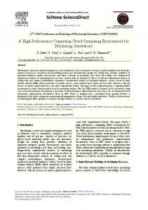
Figure 4.3. A generic block diagram of a distributed-memory SIMD machine.

limitations, they are so much cheaper that the classical vector processors are outcompeted.

4. Distributed-memory SIMD machines Machines of the DM-SIMD type are sometimes also known as processor-array machines (?). Because the processors of these machines operate in lock-step, i.e., all processors execute the same instruction at the same time (but on different data items), no synchronisation between processors is required. This greatly simplifies the design of such systems. A control processor issues the instructions that are to be executed by the processors in the processor array. Presently, no commercially available machines of the processor-array type are marketed. However, because of the shrinking size of devices on a chip, it may be worthwhile to locate a simple processor with its network components on a single chip thus making processor-array systems economically viable again. In fact, common Graphical Processing Units (GPUs) share many characteristics with processor array systems. This is the reason we still discuss this type of system. DM-SIMD machines use a front-end processor to which they are connected by a data path to the control processor. Operations that cannot be executed by the processor array or by the control processor are offloaded to the frontend system. For instance, I/O may be through the front-end system, by the processor array machine itself, or by both. Figure ?? shows a generic model of a DM-SIMD machine of which actual models will deviate to some degree. Figure ?? might suggest that all processors in such systems are connected in a 2-D grid and indeed, the interconnection topology of this type of machine always includes the 2-D grid. As opposing ends of each grid line are also always connected, the topology is rather that of a torus. This is not the only interconnection scheme: They might also be connected in 3-D, diagonally, or in more complex structures. It is possible to exclude processors in the array from executing an instruc-


9

tion on certain logical conditions, but this means that during the time of this instruction these processors are idle (a direct consequence of the SIMDtype operation) which immediately lowers the performance. Another factor that may adversely affect the speed occurs when data required by processor i resides in the memory of processor j — in fact, as this occurs for all processors at the same time, this effectively means that data will have to be permuted across the processors. To access the data in processor j, the data will have to be fetched by this processor and then sent through the routing network to processor i. This may be fairly time consuming. For both reasons mentioned, DM-SIMD machines are rather specialised in their use when one wants to employ their full parallelism. Generally, they perform excellently on digital signal and image processing, and on certain types of Monte Carlo simulations where virtually no data exchange between processors is required, and exactly the same type of operations are done on massive data sets with a size that can be made to fit comfortably in these machines. They will also perform well on gene-matching type of applications. The control processor as depicted in Figure ?? may be more or less intelligent. It issues the instruction sequence that will be executed by the processor array. In the worst case (that means a less autonomous control processor) when an instruction is not fit for execution on the processor array (e.g., a simple print instruction) it might be offloaded to the front-end processor which may be much slower than execution on the control processor. In the case of a more autonomous control processor this can be avoided thus saving processing interrupts both on the front-end and on the control processor. Most DM-SIMD systems have the ability to handle I/O independently from the front-end processors. This is favourable because the communication between the front-end and back-end systems is avoided. A (specialised) I/O device for the processor-array system is generally much more efficient in providing the necessary data directly to the memory of the processor array. Especially for very data-intensive applications like radar and image processing such I/O systems are very important. A feature that is peculiar to this type of machines is that the processors are sometimes of a very simple bit-serial type, i.e., the processors operate on the data items bit-wise, irrespective of their type. So, e.g., operations on integers are produced by software routines on these simple bit-serial processors which takes at least as many cycles as the operands are long. So, a 32-bit integer result will be produced two times faster than a 64-bit result. For floatingpoint operations a similar situation holds, be it that the number of cycles required is a multiple of that needed for an integer operation. As the number of processors in this type of system is mostly large (1024 or larger, the Quadrics Apemille was a notable exception, however), the slower operation on floating-point numbers can be often compensated for by their number, while the cost per processor is quite low as compared to full floating-point

10

J.J. Dongarra & A.J. van der Steen 0

1

2

3

4

5

6

7 0 1 2 3

I n

(a)

4 5

Shared Memory System

6 7

CPU

CPU

CPU

Out

Network (b)

Memory

(b): 1ïnetwork

(c): Central Databus

(c)

0

1

1

2

2

3

3

4

4

5

5

6

6

7

7

0

0

1

1

2

(a): Crossbar

0

2

3

3

4

4

5

5

6

6

7

7

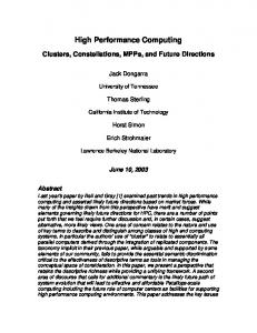
Figure 5.4. Some examples of interconnection structures used in shared-memory MIMD systems.

processors. In some cases, however, floating-point co-processors were added to the processor-array. Their number was 8–16 times lower than that of the bit-serial processors because of the cost argument. An advantage of bitserial processors is that they may operate on operands of any length. This is particularly advantageous for random number generation (which often boils down to logical manipulation of bits) and for signal processing because in both cases operands of only 1–8 bits are abundant. because, as mentioned, the execution time for bit-serial machines is proportional to the length of the operands, this may result in significant speedups. Presently there are no DM-SIMD systems on the market but some types of computational accelerators (see section ??) share many characteristics with DM-SIMD systems that have existed until shortly. We will briefly discuss some properties of these accelerators later.

5. Shared-memory MIMD machines In Figure ?? already one subclass of this type of machines was shown. In fact, the single-processor vector machine discussed there was a special case of a more general type. The figure shows that more than one FPU and/or VPU may be possible in one system. The main problem one is confronted with in shared-memory systems is that of the connection of the CPUs to each other and to the memory. As


11

more CPUs are added, the collective bandwidth to the memory ideally should increase linearly with the number of processors, while each processor should preferably communicate directly with all others without the much slower alternative of having to use the memory in an intermediate stage. Unfortunately, full interconnection is quite costly, growing with O(n2 ) while increasing the number of processors with O(n). So, various alternatives have been tried. Figure ?? shows some of the interconnection structures that are (and have been) used. As can be seen from the Figure, a crossbar uses n2 connections, an Ωnetwork uses n log2 n connections while with the central bus there is only one connection. This is reflected in the use of each connection path for the different types of interconnections: for a crossbar each data path is direct and does not have to be shared with other elements. In case of the Ωnetwork there are log2 n switching stages and as many data items may have to compete for any path. For the central data bus all data have to share the same bus, so n data items may compete at any time. The bus connection is the least expensive solution, but it has the obvious drawback that bus contention may occur, thus slowing down the computations. Various intricate strategies have been devised using caches associated with the CPUs to minimise the bus traffic. This leads however to a more complicated bus structure which raises the costs. In practice it has proved to be very hard to design buses that are fast enough, especially where the speed of the processors has been increasing very quickly and it imposes an upper bound on the number of processors thus connected that in practice appears not to exceed a number of 10-20. In 1992, a new standard (IEEE P896) for a fast bus to connect either internal system components or to external systems was defined. This bus, called the Scalable Coherent Interface (SCI) provides a point-to-point bandwidth of 200-1,000 MB/s. It has been used in the HP Exemplar systems, but also within a cluster of workstations as offered by SCALI. The SCI is much more than a simple bus and it can act as the hardware network framework for distributed computing, see (?). It has now been effectively superseded by InfiniBand, however (see section ??). A multi-stage crossbar is a network with a logarithmic complexity and it has a structure which is situated somewhere in between a bus and a crossbar with respect to potential capacity and costs. The Ω-network as depicted in Figure ?? is an example. Commercially available machines like the IBM eServer p575, the SGI Altix UV, and many others use(d) such a network structure, but a number of experimental machines also have used this or a similar kind of interconnection. The BBN TC2000 that acted as a virtual shared-memory MIMD system used an analogous type of network (a Butterfly-network) and it is likely that new machines will use it, especially as the number of processors grows. For a large number of processors the n log2 n

12


connections quickly become more attractive than the n2 used in crossbars. Of course, the switches at the intermediate levels should be sufficiently fast to cope with the bandwidth required. Obviously, not only the structure but also the width of the links between the processors is important: a network using 16-bit parallel links will have a bandwidth which is 16 times higher than a network with the same topology implemented with serial links. Until recently multi-processor vectorprocessors used crossbars. This was feasible because the maximum number of processors within in a system node was small (16 at most). In the late Cray X2 the number of processors had increased so much, however, that it had to change to a logarithmic network topology (see section ??). It not only becomes harder to build a crossbar of sufficient speed for the larger numbers of processors, the processors themselves generally also increase in speed individually, doubling the problems of making the speed of the crossbar match that of the bandwidth required by the processors. Whichever network is used, the type of processors in principle could be arbitrary for any topology. In practice, however, bus structured machines cannot support vector processors as the speeds of these would grossly mismatch with any bus that could be constructed with reasonable costs. All available bus-oriented systems use RISC processors as far as they still exist. The local caches of the processors can sometimes alleviate the bandwidth problem if the data access can be satisfied by the caches thus avoiding references to the memory. The systems discussed in this subsection are of the MIMD type and therefore different tasks may run on different processors simultaneously. In many cases synchronisation between tasks is required and again the interconnection structure is very important here. Some Cray vectorprocessors in the past employed special communication registers within the CPUs (the X-MP and Y-MP/C series) by which they could communicate directly with the other CPUs they have to synchronise with. This is, however, not practised anymore as it is viewed too costly a feature. The systems may also synchronise via the shared memory. Generally, this is much slower but it can still be acceptable when the synchronisation occurs relatively seldom. Of course, in bus-based systems communication also has to be done via a bus. This bus is mostly separated from the data bus to ensure a maximum speed for the synchronisation.

6. Distributed-memory MIMD machines The class of DM-MIMD machines represents undoubtedly the largest fraction in the family of high-performance computers. A generic diagram is given in Figure ??. The figure shows that within a computational node A, B, etc., a number of processors (four in this case) draw on the same local

HPC computers: Status and outlook Node A Processors

Node B Processors

Memory

Memory

13

Network

Figure 6.5. Generic diagram of a DM-MIMD machine.

memory and that the nodes are connected by some network. Consequently, when a processor in node A needs data present in node B this has to be accessed through the network. Hence the characterisation of the system as being of the distributed memory type. The vast majority of all HPC systems today are a variation of the model shown in Figure ??. This type of machines is more difficult to deal with than shared-memory machines and DM-SIMD machines. The latter type of machines are processorarray systems in which the data structures that are candidates for parallelisation are vectors and multi-dimensional arrays that are laid out automatically on the processor array by the system software. For shared-memory systems the data distribution is completely transparent to the user. This is generally quite different for DM-MIMD systems where the user has to distribute the data over the processors, and also the data exchange between processors has to be performed explicitly when using the so-called message passing parallelisation model (which is the case in the vast majority of programs). The initial reluctance to use DM-MIMD machines seems to have decreased. This is partly due to the now existing standard for communication software ((?, ?, ?)) and partly because, at least theoretically, this class of systems is able to outperform all other types of machines. Alternatively, instead of message passing, a Partitioned Global Address Space parallelisation model may be used with a programming language like UPC (?) or Co-Array Fortran (?). In this case one still has to be aware where the relevant data are, but no explicit sending/receiving between processors is necessary. This greatly simplifies the programming but the compilers are still either fairly immature or even in an experimental stage which does not always guarantee a great performance to say the least. The advantages of DM-MIMD systems are clear: the bandwidth problem that haunts shared-memory systems is avoided because the bandwidth scales up automatically with the number of processors. Furthermore, the speed of

14


the memory which is another critical issue with shared-memory systems (to get a peak performance that is comparable to that of DM-MIMD systems, the processors of the shared-memory machines should be very fast and the speed of the memory should match it) is less important for the DM-MIMD machines, because more processors can be configured without the aforementioned bandwidth problems. Of course, DM-MIMD systems also have their disadvantages: The communication between processors is slower than in SM-MIMD systems, and so, the synchronisation overhead, in the case of communicating tasks, is generally orders of magnitude higher than in shared-memory machines. Moreover, the access to data that are not in the local memory belonging to a particular processor have to be obtained from non-local memory (or memories). This again is very slow compared to local data access. When the structure of a problem dictates a frequent exchange of data between processors and/or requires many processor synchronisations, it may well be that only a very small fraction of the theoretical peak speed can be obtained. As already mentioned, the data and task decomposition are factors that mostly have to be dealt with explicitly, which may be far from trivial. It will be clear from the paragraph above that also for DM-MIMD machines both the topology and the speed of the data paths are crucial for the practical usefulness of a system. Again, as in the section on SM-MIMD systems, the richness of the connection structure has to be balanced against the costs. Of the many conceivable interconnection structures, only a few are popular in practice. One of these is the so-called hypercube topology as depicted in Figure ?? (a). A nice feature of the hypercube topology is that for a hypercube with 2d nodes the number of steps to be taken between any two nodes is at most d. So, the dimension of the network grows only logarithmically with the number of nodes. In addition, theoretically, it is possible to simulate any other topology on a hypercube: trees, rings, 2-D and 3-D meshes, etc. In practice, the exact topology for hypercubes does not matter too much anymore because all systems in the market today employ what is called “wormhole routing” or variants thereof. This means that a message is sent from node i to node j, a header message is sent from i to j, resulting in a direct connection between these nodes. As soon as this connection is established, the proper data is sent through this connection without disturbing the operation of the intermediate nodes. Except for a small amount of time in setting up the connection between nodes, the communication time has become fairly independent of the distance between the nodes. Of course, when several messages in a busy network have to compete for the same paths, waiting times are incurred as in any network that does not directly connect any processor to all others and often rerouting strategies are employed to circumvent busy links if the connecting network supports it. Also the network

15


d=1 1=1

d=2 1=2

d=3 1=3

d=4 1=4

(a) Hypercubes, dimension 1ï4.

(b) A 128ïway fat tree.

Figure 6.6. Some often used networks for DM machine types.

nodes themselves have become quite powerful and, depending on the type of network hardware may send and rerout message packages in a way that minimises contention. Another cost-effective way to connect a large number of processors is by means of a fat tree. In principle a simple tree structure for a network is sufficient to connect all nodes in a computer system. However, in practice it turns out that, near the root of the tree, congestion occurs because of the concentration of messages that first have to traverse the higher levels in the tree structure before they can descend again to their target nodes. The fat tree amends this shortcoming by providing more bandwidth (mostly in the form of multiple connections) in the higher levels of the tree. One speaks of a N -ary fat tree when the levels towards the roots are N times the number of connections in the level below it. An example of a quaternary fat tree

16


with a bandwidth in the highest level that is four times that of the lower levels is shown in Figure ?? (b). A number of massively parallel DM-MIMD systems seem to favour a 2or 3-D mesh (torus) structure. The rationale for this seems to be that most large-scale physical simulations can be mapped efficiently on this topology and that a richer interconnection structure hardly pays off. However, some systems maintain (an) additional network(s) besides the mesh to handle certain bottlenecks in data distribution and retrieval (?). Also on IBM’s BlueGene systems this philosophy has been followed. A large fraction of systems in the DM-MIMD class employ crossbars. For relatively small amounts of processors (in the order of 64) this may be a direct or 1-stage crossbar, while to connect larger numbers of nodes multi-stage crossbars are used, i.e., the connections of a crossbar at level 1 connect to a crossbar at level 2, etc., instead of directly to nodes at more remote distances in the topology. In this way it is possible to connect many thousands of nodes through only a few switching stages. In addition to the hypercube structure, other logarithmic complexity networks like Butterfly, Ω, or shuffle-exchange networks and fat trees are often employed in such systems. As with SM-MIMD machines, a node may in principle consist of any type of processor (scalar or vector) for computation or transaction processing together with local memory (with or without cache) and, in almost all cases, a separate communication processor with links to connect the node to its neighbours. Nowadays, the node processors are mostly off-the-shelf RISC processors sometimes enhanced by vector processors. A problem that is peculiar to DM-MIMD systems is the mismatch of communication vs. computation speed that may occur when the node processors are upgraded without also speeding up the intercommunication. In many cases this may result in turning computational-bound problems into communication-bound problems.

7. ccNUMA machines As already mentioned in the introduction, a trend can be observed to build systems that have a rather small (up to 16) number of processors that are tightly integrated in a cluster, a Symmetric Multi-Processing (SMP) node. The processors in such a node are virtually always connected by a 1-stage crossbar while these clusters are connected by a less costly network. Such a system may look as depicted in Figure ??. Note that in Figure ?? all CPUs in a cluster are connected to a common part of the memory. (Figure ?? looks functionally identical to Figure ??, however, there is a difference that cannot be expressed in the figure: all memory is directly accessible by all processors without the necessity to transfer the data explicitly).

17

HPC computers: Status and outlook Proc.

Proc.

Proc.

Mem. Proc.

Proc.

Proc.

Mem. Proc.

Proc.

Proc. Mem.

Proc.

Proc.

Proc.

Node

Interconnection Network

Peripherals

Figure 7.7. Block diagram of a system with a “hybrid” network: clusters of four CPUs are connected by a crossbar. The clusters are connected by a less expensive network, e.g., a Butterfly network.

The most important ways to let the SMP nodes share their memory are S-COMA (Simple Cache-Only Memory Architecture) and ccNUMA, which stands for Cache Coherent Non-Uniform Memory Access. Therefore, such systems can be considered as SM-MIMD machines. On the other hand, because the memory is physically distributed, it cannot be guaranteed that a data access operation always will be satisfied within the same time. In S-COMA systems the cache hierarchy of the local nodes is extended to the memory of the other nodes. So, when data is required that does not reside in the local node’s memory it is retrieved from the memory of the node where it is stored. In ccNUMA this concept is further extended in that all memory in the system is regarded (and addressed) globally. So, a data item may not be physically local but logically it belongs to one shared address space. Because the data can be physically dispersed over many nodes, the access time for different data items may well be different which explains the term non-uniform data access. The term “Cache Coherent” refers to the fact that for all CPUs any variable that is to be used must have a consistent value. Therefore, it must be assured that the caches that provide these variables are also consistent in this respect. There are various ways to ensure that the caches of the CPUs are coherent. One is the snoopy bus protocol in which the caches listen in on transport of variables to any of the CPUs and update their own copies of these variables if they have them and are requested by a local CPU. Another way is the directory memory, a special part of memory which enables the caches to keep track of all the copies of variables and of their validity. Presently, no commercially available machine uses the S-COMA scheme. By contrast, there are several popular ccNUMA systems (like Bull’s bullx R422 series, HP Superdome, and SGI Ultraviolet) that are commercially available. An important characteristic of NUMA machines is the NUMA

18


factor. This factor shows the difference in latency for accessing data from a local memory location as opposed to a non-local one. Depending on the connection structure of the system the NUMA factor for various parts of a system can differ from part to part: accessing data from a neighbouring node will be faster than from a distant node in which possibly a number of stages of a crossbar must be traversed. So, when a NUMA factor is mentioned, this is mostly for the largest network cross-section, i.e., the maximal distance between processors. Since the appearance of the multi-core processors the, ccNUMA phnomenon also manifests itself within processors with multiple cores: first and second level cache belong to a particular core and therefore when another core needs data that does not resides in its own cache, it has to retrieve it via the complete memory hierarchy of the processor chip. This is typically orders of magnitude slower than when it can be fetched from its local cache. For all practical purposes we can classify these systems as being SMMIMD machines also because special assisting hardware/software (such as a directory memory) has been incorporated to establish a single system image although the memory is physically distributed.

8. Clusters The adoption of clusters, collections of workstations/PCs connected by a local network, has virtually exploded since the introduction of the first Beowulf cluster in 1994. The attraction lies in the (potentially) low cost of both hardware and software and the control that builders/users have over their system. The interest for clusters can be seen for instance from the IEEE Task Force on Cluster Computing (TFCC) which reviews on a regular basis the current status of cluster computing (?). Also, books that describe how to build and maintain clusters have greatly added to their popularity (?, ?). As the cluster scene has become a mature and attractive market, large HPC vendors as well as many start-up companies have entered the field and offer more or less ready out-of-the-box cluster solutions for those groups that do not want to build their cluster from scratch (hardly anyone these days). The number of vendors that sell cluster configurations has become so large that it is not possible to include all their products in this report. In addition, there is generally a large difference in the usage of clusters and they are more often used for capability computing while the integrated machines primarily are used for capacity computing. The first mode of usage meaning that the system is employed for one or a few programs for which no alternative is readily available in terms of computational capabilities. The second way of operating a system is in employing it to the full by using the most of its available cycles by many, often very demanding, applications and users. Traditionally, vendors of large supercomputer systems have learned


19

to provide for this last mode of operation as the precious resources of their systems were required to be used as effectively as possible. By contrast, Beowulf clusters used to be mostly operated through the Linux operating system (a small minority using Microsoft Windows) where these operating systems either missed the tools or these tools were relatively immature to use a cluster well for capacity computing. However, as clusters become on average both larger and more stable, there is a trend to use them also as computational capacity servers too, particularly because nowadays there is a plethora of cluster management and monitoring tools. In (?) the article is looked at some of the aspects that are necessary conditions for this kind of use like available cluster management tools and batch systems. The systems assessed then are now quite obsolete but many of the conlusions are still valid: An important, but not very surprising conclusion was that the speed of the network is very important in all but the most compute bound applications. Another notable observation was that using compute nodes with more than 1 CPU may be attractive from the point of view of compactness and (possibly) energy and cooling aspects, but that the performance can be severely damaged by the fact that more CPUs have to draw on a common node memory. The bandwidth of the nodes is in this case not up to the demands of memory intensive applications. As cluster nodes have become available with 4–8 processors where each processor also may have up to 12 processor cores, this issue has become all the more important and one might have to choose for capacity-optimised nodes with more processors but less bandwidth/processor core or capabilityoptimised nodes that contain less processors per node but have a higher bandwidth available for the processors in the node. This choice is not particular to clusters (although the phenomenon is relatively new for them), it also occurs in the integrated ccNUMA systems. Interestingly, as already remarked in the previous section, in clusters the ccNUMA memory access model is turning up now in the cluster nodes, as for the larger nodes, it is not possible anymore to guarantee symmetric access to all data items for all processor cores (evidently, for a core, a data item in its own local cache will be available more quickly than for a core in another processor). Fortunately, there is nowadays a fair choice of communication networks available in clusters. Of course Gigabit Ethernet or 10 Gigabit Ethernet are always possible, which are attractive for economic reasons, but have the drawback of a high latency (≈ 10–40 µs). Alternatively, there are networks that operate from user space at high speed and with a latency that approaches these of the networks in integrated systems. These will be discussed in section ??.

20


9. Processors In comparison to 10 years ago the processor scene has become drastically different. While in the period 1980–1990, the proprietary processors and in particular the vectorprocessors were the driving forces of the supercomputers of that period, today that role has been taken over by common off-the-shelf processors. In fact there are only two companies left that produce vector systems while all other systems that are offered are based on RISC CPUs or x86-like ones. Therefore it is useful to give a brief description of the main processors that populate the present supercomputers and look a little ahead to the processors that will follow in the coming year. Still, we will be a bit more conservative in this section than in the description of the systems in general. The reason is processors are turned out at a tremendous pace while planning ahead for next generations takes years. We therefore tend to stick to the really existing components in this section or when already a β version of a processor is being evaluated. The RISC processor scene has shrunken significantly in the last few years. The Alpha and PA-RISC processors have disappeared in favour of the Itanium processor product line and, interestingly, the MIPS processor line that appeared and disappeared again as they were used in the highly interesting SiCortex systems. Unfortunately SiCortex had to close down recently and with it the MIPS processors. In addition, the Itanium processor is not used in HPC anymore. The disappearance of RISC processor families demonstrates a trend that is both worrying and interesting: worrying because the diversity in the processor field is decreasing severely and, with it, the choice for systems in this sector. On the other hand there is the trend to enhance systems having runof-the-mill processors with special-purpose add-on processors in the form of FPGAs or other computational accelerators because their possibilities in performance, price level, power consumption, and ease of use has improved to a degree that they offer attractive alternatives for certain application fields. The notion of “RISC processor” altogether has eroded somewhat in the sense that the processors that execute the Intel x86 (CISC) instruction set now have most of the characteristics of a RISC processor. Both the AMD and Intel x86 processors in fact decode the CISC instructions almost entirely into a set of RISC-like fixed-length instructions. Furthermore, both processor lines feature out-of-order execution, both are able to address and deliver results natively in 64-bit length, and the bandwidth from memory to the processor core(s) have become comparable to those of RISC/EPIC processors. A distinguishing factor is still the mostly much larger set of registers in the RISC processors. Another notable development of the last few years are the placement of

21

HPC computers: Status and outlook Core 0

Core 1

Core 2

Core 3

Core 4

Core 5

Core 0

Core 1

Core 2

Core 3

6 MB L3 Cache

6 MB L3 Cache

System Request Interface

System Request Interface

Crossbar

Memory Controllers

To/from DDR3 1333 MHz memory 7.2 GB/s/link (full duplex) 14.4 GB/s aggregate

Core 4

Core 5

Crossbar

HyperTransport 3.1

HyperTransport 3.1

4 GB/cycle/link 51.2 GB/s aggregate

4 GB/cycle/link 51.2 GB/s aggregate

Memory Controllers

To/from DDR3 1333 MHz memory 7.2 GB/s/link (full duplex) 14.4 GB/s aggregate

Figure 9.8. Block diagram of an AMD Opteron Magny Cours processor.

multiple processor cores on a processor chip and the introduction of various forms of multi-threading. We will discuss these developments for each of the processors separately. There are two processors one perhaps would expect in this section but are nevertheless not discussed: the Godson 3A and the Itanium Tukwila processors. The first processor, a Chinese one, based on the MIPS architecture, is not available in any machine that is marketed now or in the near future (it is to be succeeded by the Godson 3B early next year). The newest Itanium processor does not play a role anymore in the HPC scene and is therefore also omitted. 9.1. AMD Magny-Cours All AMD processors are clones with respect to Intel’s x86 Instruction Set Architecture. The 12-core Opteron variant called ”Magny-Cours” is no exception. It became available in March 2010. It is built with a feature size of 45 nm and in fact the chip is a package containing two modified 6-core Instanbul chips running at a maximum of 2.3 GHz in the 6176 SE variant. The two chips are connected through 16-bit HyperTransport 3.1 links to each other’s L3 caches with a single-channel speed of 12.8 GB/s as shown in Figure ??. The clock frequencies of the various parts of the chip are independent and different: while the processor operates at a speed of of 2.3 GHz the HyperTransport links run at 3.2 GHz and the four memory buses (two per 6-core chip) run at only 1.8 GHz, thus limiting the maximum bandwidth between memory and the chip to only 28.8 GB/s. AMD has made this choice to limit the power consumption although the new chips accomodate DDR3 memory at a speed of 1333 MHz which means that the bandwidth potentially could have been 42.7 GB/s. Like in the Istanbul processor, the Magny-Cours processor exploits the “HT Assist” function. HT Assist sets 1 MB in the L3 cache aside that contains the position and status of the cache lines in use on

22

J.J. Dongarra & A.J. van der Steen From/to L3 cache From/to L2 cache Fetch/Decode control

Load/Store queue units Data cache

Level 1 TLB 32 entries Level 2 TLB 512 entries Branch pred. table Precode cache

Integer Future Reorder Buffer

Instruction cache 64 KB

3ïway x86 instruction decoders

64 KB

File

FPUstack map/ rename

Level 2 cache

Integer exec. unit

512 KB

Addr. generation unit FPU sched. 12 entries FPU sched. 12 entries FPU sched. 12 entries

FPU registers

SSE +

SSE

SSE /,

120 entries

L2 TLB

Figure 9.9. Block diagram of an AMD Magny-Cours processor core.

the chip. In this way the change in status of cache variables does not have to be broadcast to all cores, but can simply be read from this part of the L3 cache, thus lowering the traffic in the interconnection fabric significantly. This setup is in fact an implementation of cache coherence via directory memory as explained in section ??. Comparison experiments with the earlier Shanghai processor have shown that HT Assist can be highly beneficial thanks to more bandwidth available for operand transfer. Because the number of cores has doubled with regard to the Istanbul processor the HT Assist function has become all the more important. Although they use the x86 instruction set, the AMD processors can be regarded as full-fledged RISC processors: they support out-of-order execution, have multiple floating-point units, and can issue up to 9 instructions simultaneously. A block diagram of a processor core is shown in Figure ??. It is in effect identical to the Istanbul processor core. The six cores on the chip are connected by an on-chip crossbar. It also connects to the memory controller and, as said, to its companion chip and other processors on the board via HyperTransport. The figure shows that a core has three pairs of Integer Execution Units and Address Generation Units that via an 32-entry Integer Scheduler takes care of the integer computations and of address calculations. Both the Integer Future File and the Floating-Point Scheduler are fed by the 72-entry Reorder Buffer that receives the decoded instructions from the instruction decoders. The decoding in the Opteron core has become more efficient than in the earlier processors: SSE instructions decode now into 1 micro-operation (µop) as are most integer and floating-point instructions. In addition, a piece of hardware, called the sideband stack optimiser, has been added (not shown in the figure) that takes care of the stack manipulations in the instruction stream, thus making instruction reordering more efficient, thereby increasing the effective number of instructions per cycle. The floating-point units allow out-of-order execution of instructions via


23

the FPU Stack Map & Rename unit. It receives the floating-point instructions from the Reorder Buffer and reorders them if necessary before handing them over to the FPU Scheduler. The Floating-Point Register File is 120 elements deep on par with the number of registers as available in RISC processors 1 . The floating-point part of the processor contains three units: Floating Add and Multiply units that can work in superscalar mode, resulting in two floating-point results per clock cycle and a unit handling “miscelaneous” operations, like division and square root. Because of the compatibility with Intel’s processors, the floating-point units are also able to execute Intel SSE2/3 instructions and AMD’s own 3DNow! instructions. However, there is the general problem that such instructions are not directly accessible from higher level languages, like Fortran 90 or C(++). Both instruction sets were originally meant for massive processing of visualisation data but are increasingly used for standard dense linear algebra operations. Due to the shrinkage of technology to 45 nm each core can harbour a secondary cache of 512 KB. Because of the accomodation of DDR3 memory at a bus speed of 1333 MHz the total bandwidth (but with the limitation of the 1.8 GHz memory interface) a channel transports 7.2 GB/s or 14.4 GB/s per 6-core chip. AMD’s HyperTransport is derived from licensed Compaq technology and similar to that employed in HP/Compaq’s former EV7 processors. It allows for “glueless” connection of several processors to form multi-processor systems with very low memory latencies. The Magny-Cours processor uses the fourth generation, HyperTransport 3.1, that transfers 12.8 GB/s 16-bit wide per unidirectional link. The HyperTransport interconnection possibility makes it highly attractive for building SMP-type clusters or to couple computational accelerators (see section ??) directly to the same memory as the standard processor. 9.2. IBM POWER6 In the systems that feature IBM’s supercomputer line, the p575 series, the nodes contain the POWER6 chip as the computational engine. This will change shortly and therefore we will also discuss the POWER7 processor in section ??, but as of this paper, the POWER6 is still the processor for IBM’s high-end HPC systems. As compared to its predecessor, the POWER5+ there are quite some differences, both in the chip lay-out and in the two cores that reside on a chip. Figure ?? shows the layout of the cores, caches, and controllers on the chip. Already, there are significnant changes: instead 1

For the x86 instructions 16 registers in a flat register file are present instead of the register stack that is typical for Intel architectures.

24

J.J. Dongarra & A.J. van der Steen Chip Boundary

Processor core 1

Processor core 2

L2 cache

L2 cache

4 MB

4 MB

L3 cache controller (32 MB)

MCM: Multi Chip Module GX Bus: I/O System bus

L3 Cache 32 MB

80 GB/s

From/to other chips 80 GB/s

Fabric Controller

From/to other MCM

20 GB/s

GX Bus

GX Controller

Mem. Control.

Buffer chips

Mem. Control.

Buffer chips

75 GB/s

Memory

Figure 9.10. Diagram of the IBM POWER6 chip layout

of a 1.875 MB shared L2 cache, each core now has its own 4 MB 8-way setassociative L2 cache that operates at half the core frequency. In addition, there are 2 memory controllers that connect via buffer chips to the memory and, depending on the amount of buffer chips and data widths (both are variable) can have a data read speed ≤ 51.2 GB/s and a write speed of ≤ 25.6 GB/s, i.e., with a core clock cycle of 4.7 GHz up to 11 B/cycle for a memory read and half of that for a memory write. Furthermore, the separate busses for data and coherence control between chips are now unified with a choice of both kinds of traffic occupying 50% of the bandwidth or 67% for data and 33% for coherence control. The off-chip L3 cache has shrunk from 36 to 32 MB. It is a 16-way set-associative victim cache that operates at 1/4 of the clock speed. Also the core has changed considerably. It is depicted in Figure ??. The Memory management unit

To L2

To nonï cacheï able unit

Data cache (64 KB)

Load/store unit (2)

Memory management unit

Branch exec. unit

Instruction cache (64 KB)

Conditional register unit

General Purpose Registers (120)

Instruction Dispatch Unit

Instruction Fetch Unit

cache

Floating Point Registers (120)

BFU (2)

DFU

Fixed Point unit (2) Checkpoint Recovery unit BFU: Binary FloatingïPoint Unit DFU: Decimal FloatingïPoint Unit VMX: Vector Multimedia Extension

Figure 9.11. Block diagram of the IBM POWER6 core.

VMX


25

clock frequency has increased from 1.9 GHz in the POWER5+ to 4.7 GHz for the POWER6 (water cooled version), an increase of almost a factor 2.5 while the power consumption stayed in the same range of that of the POWER5+. This has partly come about by a technology shrink from a 90 nm to a 65 nm feature size. It also means that some features of the POWER5+ have disappeared. For instance, the POWER6 largely employs static instruction scheduling, except for a limited amount of floating-point instruction scheduling because some of these can sometimes be fit in empty slots left by division and square root operations. The circuitry required for dynamic instruction scheduling that thus could be removed has however been replaced by new units. Besides the 2 Fixed Point Units (FXUs) and the 2 Binary FloatingPoint Units (BFUs) that were already present in the POWER5+, there os now a Decimal Floating-Point Unit (DFU) and a VMX unit, akin to Intel’s SSE units for handling multimedia instructions. In fact, the VMX unit is inherited from the IBM PowerPC’s Altivec unit. The Decimal FloatingPoint Unit is IEEE 754R compliant. It is obviously for financial calculations and is hardly of consequence for HPC use. Counting only the operations of the BPUs both executing fused multipy-adds (FMAs), the theoretical peak performance in 64-bit precision is 4 flop/cycle or 18.8 Gflop/s/core. A Checkpoint Recovery Unit has been added that is able to catch faulty FXU and FPU (both binary and decimal) instruction executions and reschedule them for retrial. Because of the large variety of functional units, a separate Instruction Dispatch Unit ships the instructions that are ready for execution to the appropriate units, while a siginificant part of instruction decoding has been pushed into the Instruction Fetch Unit, including updating the Branch History Tables. The BFUs not only execute the usual floating-point instructions like add, multiply, and FMA. They also take care of division and square root operations. A new phenomenon is that integer divide and multiply operations are also executed by the BFUs again saving on circuitry and therefore power consumption. In addition, these operations can be pipelined in this way and yield a result every 2 clock cycles. The L1 data cache has been doubled in comparison to the POWER5+ and is now 64 KB like the L1 instruction cache. Both caches are 4-way set-associative. The Simultaneous Multi-Threading (SMT) that was already present in the POWER5+ has been retained in the POWER6 processor and has been improved by a higher associativity of the the L1 I and D caches and a larger dedicated L2 cache. Also, instruction decoding and dispatch are dedicated for each thread. By using SMT the cores are able to keep two process threads at work at the same time. The functional units get instructions for the functional units from any of the two threads whichever is able to fill a slot in an instruction word that will be issued to the functional units. In this

26


way a larger fraction of the functional units can be kept busy, improving the overall efficiency. For very regular computations single thread (ST) mode may be better because in SMT mode the two threads compete for entries in the caches, which may lead to trashing in the case of regular data access. Note that SMT is somewhat different from the “normal” way of multi-threading. In this case a thread that stalls for some reason is stopped and replaced by another process thread that is awoken at that time. Of course this takes some time that must be compensated for by the thread that has taken over. This means that the second thread must be active for a fair amount of cycles (preferably a few hundred cycles at least). SMT does not have this drawback but scheduling the instructions of both threads is quite complicated, especially where only very limited dynamic scheduling is possible. Because the much higher clock cycle, and the fact that the memory DIMMs are attached to each chip, it is not possible anymore to maintain a perfect SMP behaviour within a 4-chip node, i.e., it matters whether data is accessed from a chip’s own memory or from the memory of a neighbouring chip. Although the data is only one hop away there is a ccNUMA effect that one has to be aware of in multi-threaded applications. 9.3. IBM POWER7 As already remarked before, at this moment IBM is not yet offering HPC systems with the POWER7 inside. This will however occur rather soon: POWER7-based HPC systems are expected by the end of 2011. In addition, Hitachi is already offering a variant of its SR16000 system with the POWER7 processor. So, it is appropriate to discuss this chip already in this report. Figure ?? shows the layout of the cores, caches, and memory controllers on the chip. The technology from which the chips are built is identical to Chip boundary

51.2 GB/s in 38.4 GB/s out

POWER7 core

POWER7 core

POWER7 core

POWER7 core

L2 cache 256 kB 8ïway setïassoc.







POWER7 core

POWER7 core

POWER7 core

POWER7 core

OffïMCM link

DDR3 memory, 16 GB


Memory buffer chip Port 2

Memory Controller

Memory Controller

Memory buffer chip Port 1

DDR3 memory, 16 GB

L3 cache, 32 MB, eDRAM and Chip Interconnect

SMP links

51.2 GB/s in 38.4 GB/s out

I/O

MCM: MultiïChip Module

Figure 9.12. Diagram of the IBM POWER7 chip layout


27

that of the POWER6: 45 nm Silicon-On-Insulator but in all other aspects the differences with the former generation are large: firstly, the number of cores has quadrupled. Also the memory speed has increased from DDR2 to DDR3 via two on-chip memory controllers. As in earlier POWER versions the inbound and outbound bandwidth from memory to chip are different: 2 B/cycle in and 1.5 B/cycle out. With a bus frequency of 6.4 GHz and 4 in/out channels per controller this amounts to 51.2 GB/s inward and 38.4 GB/s outward. IBM asserts that an aggregate sustained bandwidth of ≈ 100 GB/s can be reached. Although this is very high in absolute terms with a clock frequency of 3.5–3.86 GHz for the processors this is no luxury. Therefore it is possible to run the chip in so-called TurboCore mode. In this case four of the 8 cores are turned off and the clock frequency is raised to 4.14 GHz thus almost doubling the bandwidth for the active cores. As one core is capable of absorbing/producing 16B/cycle when executing a fused floating multiply-add operation the bandwidth requirement of one core at 4 GHz is already 64 GB/s. So, the cache hierarchy and possible prefetching are extremely important for a reasonable occupation of the many functional units. Another new feature of the POWER7 is that the L3 cache has been moved onto the chip. To be able to do this IBM chose to implement the 32 MB L3 cache in embedded DRAM (eDRAM) instead of SRAM as is usual. eDRAM is slower than SRAM but much less bulky and because the cache is now onchip, the latency is considerably lower (about a factor of 6). The L3 cache communicates with the L2 caches that are private to each core. The L3 cache is partitioned in that it contains 8 regions of 4 MB, one region per core. Each partition serves as a victim cache for the L2 cache to which it is dedicated and in addition to the other 7 L3 cache partitions. Each chip features 5 10-B SMP links that supports SMP operation of up to 32 sockets. Also at the core level there are many differences with its predecessor. A single core is depicted in Figure ??. To begin with, the number of floatingpoint units is doubled to four, each capable of a fused multiply-add operation per cycle. Assuming a clock frequency of 3.86 GHz this means that a peak speed of 30.88 Gflop/s can be attained with these units. A feature that was omitted from the POWER6 core has been re-implemented in the POWER7 core: dynamic instruction scheduling assisted by the load and load reorder queues. As shown in Figure ?? there are two 128-bit VMX units. One of them executes vector instructions akin to the x86 SSE instructions. However there is also a VMX permute unit that can order non-contiguous operands such that the VMX execute unit can handle them. The instruction set for the VMX unit is an implementation of the AltiVec instruction set that is also employed in the PowerPC processors. There are also similarities with the POWER6 processor: the core contains a Decimal floating-point unit

28

J.J. Dongarra & A.J. van der Steen To L3/memory

L2 cache, 256 kB, 8ïway set assoc.

2nd level translation SLB 32 entr.

Predecode

Load Miss Queue

Advanced Data prefetch Unit

Condition Register Execution Unit (2)

Branch Execution Unit

TLB 512 entr.

Branch Prediction Unit

Branch Inf. Queue

Instr. Fetch Buffer Instr. Decode Instr. Dispatch

Instructions Data

Data Translation L1 Data Cache 32 kB 8ïway set assoc. Store Data Queue (2) Store Reord. Queue Load Reord. Queue

FPU (4)

Fixed Point Unit (2) Fixed Point & Load/Store Unit (2)

Unified Issue Queue

Instruction Translation L1 Instr. Cache 32 kB 4ïway set assoc. 6 instructions 8 instructions

VMX (2)

DFU

8 instructions

SLB: Segment Lookaside Buffer TLB: Translation Lookaside Buffer

Core boundary

Figure 9.13. Block diagram of the IBM POWER7 core.

(DFU) and a checkpoint recovery unit that can re-schedule operations that have failed for some reason. Another difference that cannot be shown is that the cores now support 4 SMT threads instead of 2. This will be very helpful for the large amounts of functional units to be kept busy. Eight instructions can be taken from the L1 instruction cache. The instruction decode unit can handle 6 instructions simultaneously while 8 instructions can be dispatched every cycle to the various functional units. The POWER7 core has elaborate power management features that reduces the power usage for parts that are idle for some time. There are two power-saving mode: nap mode and sleep mode. In the former the caches and TLBs stay coherent to re-activate quickly. In sleep mode, however, the caches are purged and the clock turned off. Only the mininum voltage to maintain the memory contents is applied. Obviously the wake-up time is longer in this case but the power saving can be significant. 9.4. IBM PowerPC 970MP processor A number of IBM systems are built from JS21 blades, the largest being the Mare Nostrum system at the Barcelona Supercomputing Centre. On these blades a variant of the large IBM PowerPC processor family is used, the dual core PowerPC 970MP. It is a series of dual-core processors the fastest of which has a clock cycle of 2.2 GHz. A block diagram of a processor core is given in Figure ??.

29


Core boundary

FMA, /,

Load/store unit (2)

FMA, /,

GPR (80)

Cond. Reg. Unit Branch Unit L1 Instr. cache (64 KB)

Instr. Dispatch Unit

Non Cachable Unit

Fixed Point unit (2)

Instr. Fetch Unit

L2 Directory/ Control

Core Interface Unit

PowerPC Bus

Bus Interface Unit

L2 Cache (1 MB)

To/from

FPR (80)

L1 Data cache (32 KB)

GPR: General Purpose Registers FPR: FloatingïPoint Registers VRF: Vector Register File

VRF (80)

VALU

VPERM

VALU: Vector ALU VPERM: Vector Permutation Unit

Figure 9.14. Block diagram of the IBM PowerPC 970MP core.

A peculiar trait of the processor is that the L1 instruction cache is two times larger than the L1 data cache, 64 against 32 KB. This is explained partly by the fact that up to 10 instructions can be issued every cycle to the various execution units in the core. Apart from two floating-point units that perform the usual dyadic operations, there is an AltiVec vector facility with a separate 80-entry vector register file, a vector ALU that performs (fused) multiply/add operations, and a vector permutation unit that attempts to order operands such that the vector ALU is used optimally. The vector unit was designed for graphics-like operations but works quite nicely on data for other purposes as long as access is regular and the operand type agrees. Theoretically, the speed of a core can be 13.2 Gflop/s/core when both FPUs turn out the results of a fused multiply-add and the vector ALU does the same. One PowerPC 970MP should therefore have a theoretical peak performance of 26.4 Gflop/s. The floating-point units also perform square-root and division operations. Apart from the floating-point and vector functional units, two integer fixed-point units and two load/store units are present in addition to a conditional register unit and a branch unit. The latter uses two algorithms for branch prediction that are applied according to the type of branch to be taken (or not). The success rate of the algorithms is constantly monitored. Correct branch prediction is very important for this processor as the pipelines of the functional units are quite deep: from 16 for the simplest integer operations to 25 stages in the vector ALU. So, a branch miss can be very costly. The L2 cache is integrated and has a size of 1 MB. To keep the load/store latency low, hardware-initiated prefetching from the L2 cache is possible and 8 oustanding L1 cache misses can be tolerated. The operations

30


are dynamically scheduled and may be out-of-order. In total 215 operations may be in flight simultateously in the various functional units, also due to the deep pipelines. The two cores on a chip have common arbitration logic to regulate the data traffic from and to the chip. There is no third level cache between the memory and the chip on the board housing them. This is possible because of the moderate clock cycle and the rather large L2 cache. 9.5. IBM BlueGene processors In the last few years two BlueGene types of systems have become available: the BlueGene/L and the BlueGene/P, the successor of the former. Both feature processors based on the PowerPC 400 processor family. BlueGene/L processor This processor is in fact a modified PowerPC 440 processor, which is made especially for the IBM BlueGene family. It runs at a speed of 700 MHz. The modification lies in tacking on floating-point units (FPUs)that are not part of the standard processor but can be connected to the 440’s APU bus. Each FPU contains two floating-point functional units capable of performing 64bit multiply-adds, divisions and square-roots. Consequently, the theoretical peak performance of a processor core is 2.8 Gflop/s. Figure ?? shows the embedding of two processor cores on a chip. As can be seen from the figure, the L2 cache is very small: only 2 KB divided in a read and a write part. In fact it is a prefetch and store buffer for the rather large L3 cache. The bandwidth to and from the prefetch buffer is high, 16 B/cycle to the CPU and 8 B/cycle to the L2 buffer. The memory resides off-chip with a maximum size of 512 MB. The data from other nodes are transported through the L2 buffer, bypassing the L3 cache in first instance. BlueGene/P processor Like the BlueGene/L processor the BlueGene/P processor is based on the PowerPC core, the PowerPC 450 in this case at a clock frequency of 850 MHz and with similar floating-point enhancements as applied to the PPC 440 in the BlueGene/L. The BlueGene/P node contains 4 processor cores which brings the peak speed to 13.6 Gflop/s/node. The block diagram in Figure ?? shows some details. As can be seen from the Figure the structure of the core has not changed much with respect to the BlueGene/L. The relative bandwidth from the L2 cache has been maintained: 16 B/cycle for reading and 8 B/cycle for writing. In contrast to the BlueGene/L, the cores operate in SMP mode through multiplexing switches that connect pairs of cores to the two 4 MB L3 embedded DRAM chips. So, the L3 size has doubled. Also, the memory per node has increased to 2 GB from 512 MB.

31

HPC computers: Status and outlook L1 instr. L1 data cache cache 32 KB 32 KB

L1 instr. L1 data cache cache 32 KB 32 KB

PPC440 CPU + I/O Proc.


Snoop bus

FPU: /, +, , (2 )

5.5 GB/s

5.5 GB/s

Prefetch buffer 2 KB L2R L2W 11 GB/s

Multiported shared SRAM buffer Shared directory for embedded DRAM

Embedded DRAM/L3 cache 4 MB

5.5 GB/s To/from memory

22 GB/s

11 GB/s

11 GB/s

Prefetch buffer 2 KB L2R L2W 11 GB/s

5.5 GB/s

5.5 GB/s

FPU: /, +, , (2 )

Torus Tree Global network network interrupt

Figure 9.15. Block diagram of an IBM BlueGene/L processor chip.

9.6. Intel Xeon Two variants of Intel’s Xeon processors are employed presently in HPC systems (clusters as well as integrated systems): The Nehalem EX, officially the X7500 chip series, and the Westmere EP, officially the X5600 series. Although there is a great deal of communality they are sufficiently different to discuss both processors separately.

32

J.J. Dongarra & A.J. van der Steen L1 instr. L1 data cache cache 32 KB 32 KB







PPC450 CPU + I/O Proc. 7 GB/s

7 GB/s

7 GB/s

7 GB/s

7 GB/s

7 GB/s

7 GB/s

7 GB/s

7 GB/s

FPU: /, +, , (2 )

FPU: /, +, , (2 )

FPU: /, +, , (2 )

FPU: /, +, , (2 )

Prefetch buffer 2 KB L2R L2W




Multiplexing switch

Multiplexing switch

14 GB/s/link

14 GB/s/link Embedded DRAM/L3 cache 4 MB

Embedded DRAM/L3 cache 4 MB

DDR2 controller

DDR2 controller 13.6 GB/s

Tree network 3 6.8 Gb/s

DMA Torus network

Global interrupt

6 3.4 Gb/s

6 3.5 Gb/s

To/From Memory

Figure 9.16. Block diagram of an IBM BlueGene/P processor chip.

Nehalem EX The Nehalem EX became available in March 2010 or, more officially, the X7500 series of processors can be regarded as a heavy-duty server extension of the earlier Nehalem EP (X5500) processor. As such it has double the amount of cores, eight, and the number of QPI links also doubled to four to enable the connection to other processors on a server board. In addition the bandwidth is raised because the number of memory interfaces has increased from three to four. As the bandwidth per memory channel is 10.833 GB/s the aggregate bandwidth of the chip is 43.3 MB/s. The Nehalem EX is employed in SGI’s Altix UV systems and a variety of products from cluster vendors. Below we show the block diagram of the processor core which is in fact identical to that of the Nehalem EP and built in the same 45 nm technology. A block diagram of the core is given in Figure ?? while the layout of an 8-core chip is shown in Figure ??. To stay backwards compatible with the x86 (IA-32) Instruction Set Architecture, which comprises a CISC instruction set, Intel developed a modus in which these instructions are split in so-called micro operations (µ-ops) of fixed length that can be treated in the way RISC processors do. In fact the µ-ops constitute a RISC operation set. The price to be payed for this much more efficient instruction set is an extra decoding stage. Branch prediction has been improved and also a second level TLB cache been added. As in the earlier Core architecture 4 µ-ops/cycle and some macro-instructions as well as some µ-ops can be fused, resulting in less instruction handling, easier scheduling and better instruction throughput because these fused op-

33

HPC computers: Status and outlook 8B/

Instruction fetch & predecode

Instruction TLB

µ op queue

Microcode ROM

Allocator/Register renamer

cycle

8B/ cycle

L1 Instruction cache (32 KB)

Trace cache 12 K µ ops Retirement Unit

L3 Cache (24 MB)

P0

P1

P2

Load unit

P3

Store Address unit

L1 Data cache (32 KB)

32 B/cycle

P4

Store Data unit

P5

ALU & shift Branch FP Shuff SSE Int ALU & shuffle

Execution Engine

ALU ALU & shift & LEA FP FP + Compl. FP / Integer SSE Int ALU & SSE Int shuffle

L2 TLB

To/from memory 43.833 GB/s

µ ops)

Unified Reservation Station (32

L2 Cache (256 KB)

32 B/ cycle

Data TLB

Core

P x, x = 0,...,5 = Port x LEA = Load Effective Address

Figure 9.17. Block diagram of an Intel Nehalem processor core. Chip boundary Core

Core

Core

Core

Core

Core

Core

Core

0

1

2

3

4

5

6

7

3 MB 3 MB 3 MB 3 MB 3 MB 3 MB 3 MB 3 MB

Sys. Interface

Sys. Interface

Router

Mem. Contr.

QPI Contr.

Mem. Contr. 10.83 GB/s

10.83 GB/s

QPI

25.6 GB/s

10.83 GB/s

10.83 GB/s Memory

Memory

Memory

Memory

Memory

Memory

Memory

Memory

Memory

Memory

Memory

Memory

Figure 9.18. Diagram of a Nehalem EX processor.

34


erations can be executed in a single cycle. In the Nehalem, 2 additional µ-ops can be fused in comparison to the Core architecture. As can be seen in Figure ?? the processor cores have an execution trace cache which holds partly decoded instructions of former execution traces that can be drawn upon, thus foregoing the instruction decode phase that might produce holes in the instruction pipeline. The allocator dispatches the decoded instructions, the µ-ops, to the unified reservation station that can issue up to 6 µ-ops/cycle to the execution units, collectively called the Execution Engine. Up to 128 µ-ops can be in flight at any time. Figure ?? shows that port 0 and port 5 drive two identical Integer ALUs as well as Integer SSE units. Port 0, 1, and 5 take care of the various floating-point operations. The two integer Arithmetic/Logical Units at port 0 and 5 are kept simple in order to be able to run them at twice the clock speed. In addition there is an ALU at port 1 for complex integer operations that cannot be executed within one cycle. The floating-point units also contain additional units that execute the Streaming SIMD Extensions 4 (SSE4) repertoire of instructions, an instruction set of more than 190 instructions, that was initially meant for vector-oriented operations like those in multimedia, and 3-D visualisation applications, but is also an advantage for regular vector operations as occur in dense linear algebra. The length of the operands for these units is 128 bits. The Intel compilers have the ability to address the SSE4 units. This enables in principle much higher floating-point performance. Port 2, 3, and 4 serve the Load unit, the Store Address unit, and the Store Data unit, respectively. A notable enhancement that cannot be shown in the figures is that the Nehalem (again) supports multi-threading, much in the style of IBM’s simultaneous multithreading, and is called Hyperthreading by Intel. Hyperthreading was earlier introduced in the Pentium 4 but disappeared in later Intel processors because the performance gain was very low. Now with a much higher bandwidth and larger caches speedups of more than 30% for some codes have been observed with Hyperthreading. Another feature that cannot be shown is the so-called Turbo Mode. This means that the clock cycle can be raised from its nominal speed (2.91 GHz for the fastest variant) by steps of 133 MHz to over 3 GHz as long as the thermal envelope of the chip is not exceeded. So, when some cores are relatively idle other cores can take advantage by operating at a higher clock speed. The L1 caches have the same size as in the Nehalem’s predecessor, but the L2 cache is much smaller: 256 KB instead of 6 MB. It is much faster however and able to deliver requested data in 10 cycles or less. The Nehalems feature a common L3 cache that is used by all eight cores in the EX version. Each core has its own section of 3 MB but when data is not found in the section of a core the other sections can be searched for the missing data item(s).


35

The L3 cache is inclusive which means that it contains all data that are in the L2 and L1 cache. The consequence is that when a data item cannot be found in the L3 cache it is also not in any of the caches of the other cores, and therefore one need not search them. In Figure ?? it can be noticed that apart from the first bank of memory of ≤ 32 GB also a second and third bank are depicted, represented by dashed boxes. This means that it is indeed possible to have up to 96 GB of memory/processor. However, this can only be done at the expense of the memory bus speed: for one bank it is 1333 MB/s, for two banks it is 1066 MB/s, and for three banks only 800 MB/s. So, the latter two options may be chosen for instance for database systems that benefit from a large memory that not needs to be at the very highest speed. For HPC purposes, however, configurations with only one memory bank/processor will usually be offered. Westmere EP The Westmere EP (X5600 series) is a 32 nm technology shrink of the Nehalem EP chip. The smaller feature size is used to place 6 cores on a die. The fastest variant, the X5690 has a clock cycle of 3.46 GHz at 130 W. The structure of the core is the same as in the Nehalem processors (see Figure ??) but there are slight differences in the instruction set for the Advanced Encryption Standard (AES). The new instructions, among which is a carryless multiplication, are said to speed up the en/decryption rate by a factor of three. Also the Westmere EP supports the use of 1 GB pages. The packaging on the chip is, apart from the number of cores, identical to that of the Nehalem EP chip with exception of the shared L3 cache. The size of this is halved from 24 MB to 12 MB. The chip layout is depicted in Figure ?? 9.7. The SPARC processors Since SUN has been taken over by Oracle all processor development has been shelved. The development of the SPARC processor architecture is now in the hands of Fujitsu that advances with its own SPARC64 implementation. Fujitsu/Siemens markets its HPC servers based on the latter processor. Below we discuss the current SPARC chip that is commercially available in the Fujitsu machines. Although a follow-on processor, the SPARC64 VIII seems ready for incoporation in Japan’s 10 Petaflop/s system that is currently being built, we only discuss the SPARC64 VII here as this is the one that is commerically available. Presently it is not known when its successor will appear on the open market. The SPARC64 VII is, obviously, Fujitsu’s seventh generation of the processor. Of course, the processor must be able to execute the SPARC instruction set but the processor internals are rather different from Sun’s late

36

J.J. Dongarra & A.J. van der Steen Chip boundary Core

Core

Core

Core

Core

Core

0

1

2

3

4

5

L3 cache 12 MB

Sys. Interface

Router

QPI Contr.

Mem. Controller 10.83 GB/s

10.83 GB/s

10.83 GB/s

QPI

25.6 GB/s

Memory

Memory

Memory

Memory

Memory

Memory

Memory

Memory

Memory

Figure 9.19. Diagram of a Westmere EP processor.

implementations. Figure ?? shows a block diagram of one core of the quadcore SPARC64 VII. Core boundary

Commit Stack Entry L1 I cache 64 KB Instruction Buffer Branch Target addr. 16 KB

Instruction Word Register

Fetch port

Control registers(2) RSA

GPR (2)

RSE

GUB

RSF

FPR (2)

RSBR

FUB

RSA/RSE : Reservation stations for integer registers. RSF (A & B): Reservation stations for floatingïpoint registers. RSBS: Reservation station for Branch branch target unit. GPR: Registers for integer and address generation units (EAG and EX A & B)., FPR: Registers for floating ïpoint units (FL A & B). GUB: General register update buffer. FUB: Floatingïpoint register update buffer.

EAGïB EAGïA

Store port Store buffer

EXïB EXïA

FLïA

L1 D cache 64 KB

To L2 cache (6 MB)

Prog. counter(2)

FLïB

Figure 9.20. Block diagram of a Fujitsu SPARC64 VII processor core.

Actually, the core achitecture has not changed from the SPARC64 VI but thanks to the decrease of the feature size from 90 nm to 65 nm, now 4 cores can be placed on a chip while the highest available clock frequency is raised from 2.4 GHz to 2.52 GHz. The L1 instruction and data caches are 64 KB, two times smaller than in the SPARC64 VI core and both 2-way set-associative. This decrease in size is somewhat surprising and probably due to the technology shrink to 65 nm feature size. There is also an Instruction Buffer (IBF) that contains


37

up to 48 4-byte instructions and continues to feed the registers through the Instruction Word Register when an L1 I-cache miss has occurred. A maximum of four instructions can be scheduled each cycle and find their way via the reservation stations for address generation (RSA), integer execution units (RSE), and floating-point units (RSF) to the registers. The two general register files serve both the two Address Generation units EAG-A, and B, and the Integer Execution units EX-A and -B. The latter two are not equivalent: only EX-A can execute multiply and divide instructions. There also two floating-point register files (FPR), that feed the two Floating-Point units FL-A and FL-B. These units are different from those of Sun in that they are able to execute fused multiply-add instructions as is also the case in the POWER and Itanium processors. Consequently, a maximum of 4 floating-point results/cycle can be generated. In addition, FL-A and -B also perform divide and square root operations in contrast to the SPARC4+ that has a separate unit for these operations. Because of their iterative nature, the divide and square root operations are not pipelined. The feedback from the execution units to the registers is decoupled by update buffers: GUB for the general registers and FUB for the floating-point registers. The dispatch of instructions via the reservation stations that each can hold 10 instructions gives the opportunity of speculative dispatch: i.e., dispatching instructions of which the operands are not yet ready at the moment of dispatch but will be by the time that the instruction is actually executed. The assumption is that it results in a more even flow of instructions to the execution units. The SPARC64 VII does not have a third level cache but on chip there is a large (6 MB) unified L2 12-way set-associative write-through cache that is shared by the 4 cores in a processor as can be seen in Figure ??. Note that the system bandwidth is the highest available. For the lower end systems this bandwidth is about 8 GB/s. The Memory Management Unit (not shown in Figure ??) contains separate sets of Translation Look aside Buffers (TLB) for instructions and for data. Each set is composed of a 32-entry µTLB and a 1024-entry main TLB. The µTLBs are accessed by high-speed pipelines by their respective caches. What cannot be shown in the diagrams is that, like the IBM and Intel processors, the SPARC VII is dual-threaded per core. The type of multithreading is similar to that found in the Intel processors and is called Simultaneous Multithreading, differing from the type of multithreading present in the IBM processors but with the same name. At this moment the highest clock frequency SPARC64 available is 2.52 GHz. As already remarked, the floating-point units are capable of a fused multiply-add operation, like the POWER and Itanium processors, and so the theoretical peak performance is presently 10.08 Gflop/s/core and consequently 40.3 Gflop/s/processor.

38

J.J. Dongarra & A.J. van der Steen Chip boundary

Core 0 L2 Cache (6 MB)

L2 Cache Data Buffer

L2 tags

L2 Cache Data Buffer

System L2 Interface control

Core 2

Core 1

L2 tags

System L2 control Interface

Core 3

11.5 GB/s

Figure 9.21. Block diagram of a Fujitsu SPARC64 VII processor chip. Four cores share the L2 cache.

10. Computational accelerators In the last few years computational accelerators have emerged and have taken a firm foothold now. They come in various forms of which we will discuss some general characteristics. Accelerators are not a new phenomenon: in the 1980’s, for instance, Floating Point Systems sold attached processors like the AP120-B with a peak performance of 12 Mflop/s, easily 10 times faster than the general purpose systems they were connected to. Also the processor array machines described in section ?? could be regarded as accelerators for matrix-oriented computations in their time. A similar phenomenon is on us at the moment. HPC users never tend to be content with the performance of the machines they have at their disposal and are continuously looking for ways to speed up their calculations or parts of them. Accelerator vendors are complying to this wish and presently there is a fair amount of products that, when properly deployed, can deliver significant performance gains. The scene is roughly divided in three unequal parts: 1 Graphical cards or Graphical Processing Units (GPUs as opposed to the general CPUs). 2 General floating-point accelerators. 3 Field Programmable Gate Arrays. The appearance of accelerators is believed to set a trend in HPC computing. Namely, that the processing units should be diversified according to their abilities. Not unlike the occurence of different functional units within a CPU core2 . In a few years this will lead to hybrid systems that incorporate 2

In principle it is entirely possible to perform floating-point computations with integer functional units, but the costs are so high that no one will attempt it.


39

different processors for different computational tasks. Of course, processor vendors can choose to (attempt to) integrate such special purpose processing units within their main processor line, but for now it is uncertain if or how this will happen. When speaking of special purpose processors, i.c., computational accelerators, one should realise that they are indeed good at some specialized computations while totally unable to perform others. So, not all applications can benefit of them and those which can, not all to the same degree. Futhermore, using accelerators effectively is not at all trivial. Although the Software Development Kits (SDKs) for accelerators have improved enormously lately, for many applications it is still a challenge to obtain a significant speedup. An important factor in this is that data must be shipped in and out the accelerator and the bandwidth of the connecting bus is in most cases a severe bottleneck. One generally tries to overcome this by overlapping data transport to/from the accelerator with processing. Tuning the computation and data transport task can be cumbersome. This hurdle has been recognised by at several software companies like Acceleware, CAPS, and Rapidmind (now absorbed by Intel). They offer products that automatically transform standard C/C++ programs into a form that integrates the functionality of GPUs, multi-core CPUs (which are often also not used optimally), and, in the case of Rapidmind, of Cell processors. There is one other and important consideration that makes accelerators popular: in comparison to general purpose CPUs they are all very powereffective. Sometimes orders of magnitude when expressed in flop/Watt. Of course they will do only part of the work in a complete system but still the power savings can be considerable which is very attractive these days. We will now proceed to discuss the three classes of accelerators mentioned above. It must be realised though that the developments in this field are extremely rapid and therefore the information given here will become obsolete very fast and therefore could be of an approximate nature. 10.1. Graphical Processing Units Graphics processing is characterised by doing the same (floating-point) operation on massive amounts of data. To accommodate this way of processing, Graphical Processing Units (GPUs) consist of a large amount of relatively simple processors, fast but limited local memory, and fast internal buses to transport the operands and results. Until recently all calculations, and hence the results, were in 32-bit precision. This is hardly of consequence for graphics processing as the colour of a pixel in a scene may be a shade off without anyone noticing. HPC users often have similar computational demands as those in the graphical world: the same operation on very many data items. So, it was natural to look into GPUs with their many integrated

40


parallel processors and fast memory. The first adopters of GPUs from the HPC community therefore disguised their numerical program fragments as graphical code (e.g., by using the graphical language OpenGL) to get fast results, often with remarkable speedups. Another advantage is that GPUs are relatively cheap because of the enormous amounts that are sold for graphical use in virtually every PC. A drawback is the 32-bit precision of the usual GPU and, in some cases more important, there is no error correction available. By carefully considering which computation really needs 64-bit precision and which does not and adjusting algorithms accordingly the use of a GPU can be entirely satisfactory, however. GPU vendors have been quick in focussing on the HPC community. They tended to rename their graphics cards to GPGPU, general-purpose GPU, although the product was largely identical to the graphics cards sold in every shop. But there have also been real improvements to attract HPC users: 64-bit GPUs have come onto the market. In addition, it is no longer necessary to reformulate a computational problem into a piece of graphics code. Both ATI/AMD and NVIDIA claim IEEE 754 compatibility (being the floating-point computation standard) but neither of them support it to the full. Error correction as is usual for general purpose CPUs is coming available (see ??). There are C-like languages and runtime environments available that makes the life of a developer for GPUs much easier: for NVIDIA this is CUDA, which has become quite popular with users of these systems. AMD/ATI is concentrating on the newly defined standard OpenCL (see below). It is somewhat more cumbersome but still provides a much better alternative to emulating graphics code. When one develops a code for a particular GPU platform it cannot be transferred to another without a considerable effort in rewriting the code. This drawback is taken up by the GPU vendors (and not only them). Recently OpenCL has become available, that in principle is platform independent, thus protecting the development effort put into the acceleration of a program. Presently, Apple, ATI/AMD, Intel, NVIDIA, and PetaPath are members of the consortium that are willing to provide an OpenCL language interface. First experiences with OpenCL version 1.0 as provided by the Khronos Group showed generally low performances but one might expect that these may improve with the new enhanced release of OpenCL 1.1 as of June 2010. Another way to be (relatively) independent of the platform is to employ some language transformer. For instance, CAPS provides such transforming tools that can target different types of accelerators or multi-core CPUs. With CAPS’ product HMPP, the transformation is brought about by inserting pragmas in the C code or comment directives in Fortran code. HMPP is the only code that has the ability to accelerate Fortran code on general GPU


41

accelerators. The Portland Group sells a CUDA/Fortran compiler that only targets NVIDIA GPUs. In the following we describe some high-end GPUs that are more or less targeting the HPC community. ATI/AMD In June 2010 the latest product from ATI (now wholly owned by AMD) was announced. It is the ATI Firestream 9370 card. As the actual delivery is scheduled by AMD in the third quarter of 2010 the information about the card is scant: There is not enough information available for a block diagram but we list some of the most important features of the processor: The specifications given indicate that, per core, 2 floating-point results per Table 10.1. Some specifications for the ATI/AMD Firestream 9370 GPU Number of processors Memory (GDDR5) Clock cycle Internal memory bandwidth Peak performance (32-bit) Peak performance (64-bit) Power requirement, typical Power requirement, peak Interconnect (PCIe Gen2) ECC, Error correction Floating-point support

1600 4 GB 825 MHz ≤ 147.2 GB/s 2.64 Tflop/s 528 Gflop/s 170 W 225 W ×16, 8 GB/s No Partial (32/64-bit)

cycle can be generated, presumably the result of an add and a multiply operation. Whether these results can be produced independently or result from linked operations is not known because of the lack of information. Unlike in NVIDIA’s Fermi card, discussed below, the Firestream 9370 does not support error correction yet. So, one has to be careful in assessing the outcomes of numerically unstable calculations. Like its direct competitor, NVIDIA, ATI offers a free Software Development Kit, SDK v.2.01 which supports OpenCL 1.1, Direct X11 and ComputeX. The earlier languages like BROOK+ and the very low level CloseTo-Metal software development vehicles are no longer supported. NVIDIA NVIDIA is the other big player in the GPU field with regard to HPC. Its latest product is the Tesla C2050/C2070, also known as the ”Fermi” card.

42


A simplified block diagram is shown in Figure ??. The GigaThread Engine To GDDR5 memory

Memory Controller

PCI Express

Host Interface

Chip boundary

3 (4)

SM

Polymorph Engine

Polymorph Engine

SM Polymorph Engine

Memory Controller

Polymorph Engine

Raster Engine SM

To GDDR5 memory

3 (4)

SM

8 GB/s

Graphics Processor Cluster

Raster Engine

Memory Controller


L2 cache

Polymorph Engine

3 (4)

SM

SM

Polymorph Engine

Polymorph Engine

3 (4)

SM Polymorph Engine

Memory Controller

Memory Controller

To GDDR5 memory

SM

Raster Engine

To GDDR5 memory


Raster Engine

Memory Controller

GigaThread Engine


SM: Streaming Multiprocessor

Figure 10.22. Simplified block diagram of the NVIDIA Tesla C2050/C2070 GPU.

is able to schedule different tasks in the Streaming Multiprocessors (SMs) in parallel. This greatly improves the occupation rate of the SMs and thus the throughput. As shown in Figure ?? 3 (or 4) SMs per Graphics Processor Cluster (GPC) are present. At the moment not more than a total of 14 SMs are available, although 16 were planned. When the 40 nm production process has sufficiently improved the number of SMs may increase from 14 to the originally planned 16. A newly introduced feature is the L2 cache that is shared by all SMs. Also there is DMA support to get data from the host’s memory without having to interfere with the host CPU. The GPU memory is GDDR5 and is connected to the card via 6 64-bit wide memory interfaces for a bandwidth of about 150 GB/s. Each SM in turn harbours 32 cores that used to be named Streaming Processors (SPs) but now are called CUDA cores by NVIDIA. A diagram of an SM with some internals is given in Figure ??. Via the instruction cache 2 Warp schedulers (a warp is a bundle of 32 threads) the program threads are pushed onto the SPs. In addition each SM has 4 Special Function Units that take care of the evaluation of functions that are more complicated than profitably can be computed by the simple floating-point units in the SPs. Lastly, we list some properties of the Tesla C2050/70 in the table below. From these specifications, it can be derived that 2 32-bit floating-point results per core per cycle can be delivered. The peak power requirement given will probably be an appropriate measure for HPC workloads. A large proportion of the work being done will be from the BLAS library that is provided by NVIDIA, more specifically, the dense matrix-matrix multiplication in it. This operation occupies any computational core to the fullest


43

SM Instruction cache Warp sched.

Warp sched.

Dispatch Unit

Dispatch Unit

Register File (4096

32ïbit)

L/S SP SP SP SP L/S

L/S SP SP SP SP L/S

SFU

SFU

L/S SP SP SP SP L/S

L/S SP SP SP SP L/S L/S SP SP SP SP L/S

L/S SP SP SP SP L/S

SFU

SFU

L/S SP SP SP SP L/S

L/S SP SP SP SP L/S Network Shared Memory/L1 cache Uniform cache

L/S: Load/Store unit SM: Streaming Multiprocessor SP: Streaming Processor SFU: Special Function Unit

Figure 10.23. Diagram of a Streaming Processor of the NVIDIA Tesla C2050/C2070.

Table 10.2. Some specifications for the NVIDIA Tesla C2050/70 GPU Number of processors Memory (GDDR5), C2050 Memory (GDDR5), C2070 Internal bandwidth Clock cycle Peak performance (32-bit) Peak performance (64-bit) Power requirement, peak Interconnect (PCIe Gen2) ECC, Error correction Floating-point support

448 3 GB 6 GB ≤ 153 GB/s 1.15 GHz 1.03 Tflop/s 515 Gflop/s 238 W ×8, 4 GB/s;×16, 8 GB/s Yes Full (32/64-bit)

and will therefore consume close to the maximum of the power. As can be seen from the table the only difference between the C2050 and the C2070 is the amount of memory: the C2050 features 3 GB of GDDR5 memory while the C2070 has double that amount.

44


Like ATI, NVIDIA provides an SDK comprised of a compiler named CUDA, libraries that include BLAS and FFT routines, and a runtime system that accomodates both Linux (RedHat and SuSE) and Winodws. CUDA is a C/C++-like language with extensions and primitives that cause operations to be executed on the card instead of on the CPU core that initiates the operations. Transport to and from the card is done via library routines and many threads can be initiated and placed in appropriate positions in the card memory so as not to cause memory congestion on the card. This means that for good performance one needs knowledge of the memory structure on the card to exploit it accordingly. This is not unique to the C2050 GPU, it pertains to the ATI Firestream GPU and other accelerators as well. NVIDIA also supports OpenCL, though CUDA is at present much more popular among developers. For Windows users the NVIDIA Parallel Nsight for Visual Studio is available that should ease the optimisation of the program parts run on the cards. 10.2. General computational accelerators Although we have looked at the GPUs in the former section primarily from the point-of-view of computational accelerators, they are of course full-blown high-end graphical processors in the first place. Several vendors have developed accelerators that did not have graphical processing in mind as the foremost application to be served (although they might not be bad in this respect when compared to general CPUs). The future of the general computational accelerators is problematic: in principle it is entirely possible to make such accelerators that can compete with GPUs, or with the FPGAbased accelerators discussed in section ??, but the volume will always be much lower than that of the other two accelerator variants which is reflected in the production cost. Below we discuss two of these general accelerators for completeness’ sake, but it is doubtful that they will survive as marketable products. PetaPath PetaPath is a spin-off of ClearSpeed to position the ClearSpeed products in the HPC market. ClearSpeed works in the embedded processor sector but a main product, viz., the CSX700 processor is well equipped for HPC work. We discuss this processor in some detail below. The ClearSpeed products are in their 3rd generation. Unlike the GPUs, the ClearSpeed processors were made to operate on 64-bit floating-point data from the start and full error correction is present in them. The latest processor is the CSX700 chip that is packaged in a number of products. The most common is the e710 card that fits in a PCIe slot of any PC or server unit. A variant with a different form factor but with the same functionality


45

is the e720 card that can be put into blade servers. PetaPath also markets, apart from the separate cards, its Feynman e740 and e780 units that house 4 and 8 e720 cards and that connect to a host server by PCIe Gen. 2, 16×, i.e., at 8 GB/s. The bandwidth to the individual cards is 2 GB/s, however. As the peak performance of a single e720 card is 96 Gflop/s, the peak performances of the Feynman e740 and e780 are 384 and 768 Gflop/s, respectively. The power comsumption of the e710/e720 card is extremely low, 25 W maximal, 15 W typical. This is partly due to the low clock frequency of 250 MHz. The e710 card contains, apart from the CSX700 processor, 2 GB DDR2 SDRAM, and an FPGA that manages the data traffic to and from the card. As said, the interconnect to the host system is compliant with PCIe 8×, amounting to a bandwidth of 2 GB/s. ClearSpeed is quite complete in giving technical details. So, we are able to show a block diagram of the CSX processor in Figure ??. Two so-called Multi-Threaded Array MTAP

2 GB/s

Data Cache

Mono Controller

Instruction Cache

Control & Debug

Poly Controller

PE 0

PE 1

PE 2

PE 3

PE 95

2 GB/s Programmable I/O to DRAM

Figure 10.24. Block diagram of a ClearSpeed MTAP unit. Two of these units reside on a CSX700 chip.

Procesor (MTAP) units are located on one CSX700 chip. As can be seen an MTAP contains 96 processors (with 4 redundant ones per MTAP). They are controlled via the Poly Controller, “poly” being the indication for the data types that can be processed in parallel. The processing elements themselves are able to communicate fast between themselves via a dedicated ring network. Every cycle, a 64-bit data item can be shifted to the right or to the left through the ring. In Figure ??, we show the details of a processing element. A maximum of two 64-bit floating-point results can be generated per cycle. As one MTAP contains 96 PEs and there are 2 MTAPs on a chip, the peak performance of a CSX700 chip is 96 Gflop/s at a clock frequency of 250 MHz.

46

J.J. Dongarra & A.J. van der Steen PE x Floating Point Add

Floating Point Multiply

64 PE xï1 64

Multiply Accumulate

64

ALU

64

64 64 PE x+1

Register File (128 B) 32

PE SRAM (6 kB)

32

32

Memory address Generator (PIO)

128

Figure 10.25. Block diagram of a PE in an MTAP of a CSX700 chip. The numbers near the arrows indicate the number of bits that can be transferred per cycle.

Note the Control & Debug unit present in an MTAP. It enables debugging within the accelerator on the PE level. This is a facility that is missing in the GPUs and the FPGA accelerators we will discuss later. Also ClearSpeed employs an extended form of C, called Cn , for program development on the card. The extension is very slight, however. The keywords mono and poly are added to indicate data that should be processed serially or in parallel, respectively. Because ClearSpeed is in the accelerator trade for quite some time, the SDK is very mature. Apart from the Cn compiler already mentioned, it contains a library with a large set of the BLAS/LAPACK routines, FFTs, and Random Number generators. For dense linear algebra there is an interface that enables calling the routines from a host program in Fortran. Furthermore, a graphical debugging and optimisation tool is present that may or may not be embedded in IBM’s Eclipse Integrated Development Environment (IDE) as a plug-in. The IBM/Sony/Toshiba Cell processor The Cell processor, offically called the Cell Broadband Engine (Cell BE), was designed at least partly with the gaming industry in mind. Sony uses it for its PS3 gaming platform and to be successful it has to deliver high performance for the graphical part as well in doing a large amount of floatingpoint computation to sustain the rapidly changing scenes that occur during a game. The Cell processor is therefore not a pure graphics processor but considerably more versatile than a GPU. A testimony to this is that Mercury computers, specialised in systems for radar detection, etc., markets a product with two Cell processors, instead of dedicated DSPs (i.e., Digital Signal Processors), while Toshiba incorporates the Cell in HDTV sets and


47

considers to bring out notebooks with a Cell processor. The Cell processor is able to operate in 32-bit as well as in 64-bit floating-point mode, though there is a large performance difference: in single precision the peak speed is 204.8 Gflop/s while in double precision it is about 14 Gflop/s. From the start there was a keen interest from the HPC community. It also restarted the discussion of the necessity of using 64-bit precision calculation all the way through an application or, by reformulation some key algorithms it would not be possible to get results with acceptable accuracy when parts would be carried out in single precision (?). At least for the Cell processor this discussion has become of less importance as at present the variant is available under the name of PowerXCell 8i which is developed by IBM, probably expressly targeted at the HPC area. In the PowerXCell the speed for 64-bit precision has increased considerably to 102.4 Gflop/s, half the speed of the single precision computations. Also it is produced in 65 nm instead of 90 nm technology and it employs DDR2 memory instead of Rambus memory which is used in the original Cell processor. Figure ?? shows a diagram of this rather complicated processor. As can be seen, the processor is hybrid

PPE

6

SPE1

SPE3

SPE5

7

8

9

SPE7 10 IOIF1

FlexIO

11 EIB, 96B/cycle

XIO X2D

MIC XIO

DDR2 Memory

5

4

3

2

1

SPE0

SPE2

SPE4

SPE6

0 BEI

IOIF0

FlexIO

BEI : Broadband Engine Interface EIB : Element Interconnect Bus FlexIO : Rambus FlexIO Bus IOIF : I/O Interface MIC : Memory Interface Controller PPE : PowerPC Processor Element SPE : Synergistic Processor Element X2D : XIO to DDR2 logic

Figure 10.26. Block diagram of an IBM PowerXCell processor. The blue numbers in the figure indicate the device numbering used for delivering data via the Element Interconnect Bus.

in the sense that it contains two different kinds of processors: The PPE, which is essentially a PowerPC core as discussed in section ??, and 8 SPEs all running at a clock frequency of 3.2 GHz. The SPEs are meant to do the bulk of the computation, while the PPE takes care of operating system tasks and coordinating the work to be done by the SPEs. All devices in the processor are connected by the Element Interconnect Bus. The EIB in fact consists of four 16B wide rings that transport data in opposite directions as to minimise the distance between the devices in the processor. The devices connected to the EIB are numbered to allow data to be transferred from one device to another. Up to 96 B/cycle can be transferred, amounting to 307.2 GB/s. Although the PowerXCell uses DDR2 memory, the processor proper is designed for use with Rambus memory. This has

48


been taken care of by including the X2D device that translates the DDR memory requests into Rambus requests and vice-versa. The two I/O Interfaces are controlled through the Broadband Engine Interface (BEI). They have different functions: IOIF1 takes care of the usual external I/O devices via the IOIF protocol while IOIF0 is able to use the internal I/O protocol, BIF that is also used on the EIB rings. In this way it is possible to connect to other Cell processors. The SPEs are the computational workhorses in the Cell processor. We show the internals of an SPE in Figure ??. Roughly, there are three imporSXU

MFC

Odd pipeline

SPU Odd FixedïPoint Unit

SPU Control Unit

SPU Channel & DMA Unit

SPU Load/Store Unit

Synergistic Memory Management (SMM)

Local Store 256 kB SPU Even FixedïPoint Unit

SPU FloatingïPoint Unit

SPU Register File Unit 128ïentries

DMA Controller

Even pipeline

EIB : Element Interconnect Bus MFC: Memory Flow Controller SXU : Synergistic Execution Unit

EIB

Figure 10.27. Block diagram of an IBM PowerXCell Synergistic Processing Element (SPE).

tant parts in an SPE: the SXU (Synergistic Execution Unit) which contains the functional units for computation, load/store, and DMA-control, the Local Store that contains the local data to be operated on, and the Memory Flow Controller that in turn contains the DMA Controller and the memory management unit. As shown in Figure ??, in the SXU, the functional units are organised into an odd and an even pipeline. Two instructions can be issued every cycle, one for each of these pipelines. This also implies that one floating-point instruction can be issued per cycle. Depending on the type of the operands this can yield four 32-bit results or two 64-bit results per cycle (in the PowerXCell, in the original Cell processor a 64-bit result can be delivered every 13 cycles, hence the much lower double precision performance). Note that SPE does not have any form of cache. Rather, data is brought in from external memory by DMA instructions via the EIB. This leads to much lower memory latency when a data item is not in the Local Store. Up to 16 DMA requests can be outstanding for any of the SPEs. As all SPEs are independent up to 128 DMA requests can be in flight. Of course, this explicit memory management does not makes for easy programming. So, one must be careful in managing the data to get (close to) optimal performance. IBM has put much effort into a Software Development Kit for the Cell processor. It is freely available and, apart from the necessary compilers,


49

there is an extensive library for managing the data transport both from the PPE to the SPEs, between SPEs, initiating the processes on the SPEs, retrieving the results, and managing program overlays. As the Local Stores in the SPEs are small, the old concept of overlays has been revived again: The program is divided into units that depend on each other but do not constitute the whole program. By loading and unloading the units in the correct sequence one can still execute the total program. In addition, there are debugging and performance analysis tools. The total of the program development can be done using IBM’s IDE, Eclipse. The PowerXCell 8i won its share of fame for it’s use in the Roadrunner system at Los Alamos National Laboratory. In this system 3240 so-called triblades are connected by InfiniBand. A triblade consists of 2 QS22 blades each containing 2 PowerXCell processors and an LS21 blade with 2 Opteron processors. This configuration was the first to break the LINPACK Petaflop barrier. This fact certainly helped in increasing the interest in the Cell processor as an accelerator platform. Presently, there are many research projects under way to assess the applicability of Cell BE accelerators and to make the learning curve for employing them effectively, less steep. 10.3. FPGA-based accelerators An FPGA (Field Programmable Gate Array) is an array of logic gates that can be hardware-programmed to fulfill user-specified tasks. In this way one can devise special purpose functional units that may be very efficient for this limited task. Moreover, it is possible to configure a multiple of these units on an FPGA that work in parallel. So, potentially, FPGAs may be good candidates for the acceleration of certain applications. Because of their versatility it is difficult to specify where they will be most useful. In general, though, they are not used for heavy 64-bit precision floating-point arithmetic. Excellent results have been reported in searching, pattern matching, signal- and image-processing, encryption, etc. The clock cycle of FPGAs is low as compared to that of present CPUs: 100–550 MHz which means that they are very power effective. Vendors provide runtime environments and drivers that work with Linux as well as Windows. Tradionally, FPGAs are configured by describing the configuration by means of a hardware description language (HDL), like VHDL or Verilog. This is very cumbersome for the average programmer as one not only has to explicitly define such details as the placement of the configured devices but also the width of the operands to be be operated on, etc. This problem has been recognised by FPGA-based vendors and a large variety of programming tools and SDKs have come into existence. Unfortunately, they differ enormously in approach, and the resulting programs are far from compatible. Also for FPGA-based accelerators, like for GPUs, there is an initiative to

50


develop a unified API that will assure compatibility between platforms. The non-profit OpenFPGA consortium is heading this effort. Various working groups concentrate on, for instance, a core library, an application library, and an API definition. There is no unified way to program FPGAs platform independently, however, and it may take a long time to get there. The two big players on the FPGA market are Altera and Xilinx. However, in the accelerator business one will seldom find these names mentioned, because the FPGAs they produce are packaged in a form that makes them unusable for accelerator purposes. It is not possible to fully discuss all vendors that offer FPGA-based products. One reason is that there is a very large variety of products ranging form complete systems to small appliances housing one FPGA and the appropriate I/O logic to communicate with the outside world. To complicate matters further, the FPGAs themselves come in many variants, e.g., with I/O channels, memory blocks, multipliers, or DSPs already configured (or even fixed) and one can choose for FPGAs that have for instance a PowerPC405 embedded. Therefore we present the FPGA accelerators here only in the most global way and necessarily incomplete. In the following we will discuss products of vendors that have gone to great length to not expose their users to the use of HDLs, although for the highest benefits this not always can be avoided. Necessarily, we are here again somewhat arbitrary because this area is changing extremely rapidly.

Convey The Convey HC-1 was announced in November 2008. It is an example of the hybrid solutions that have came up to avoid the unwieldy HDL programming of FPGAs while still benefitting from their potential acceleration capabilities. The HC-1 comprises a familiar x86 front-end with a modified Centos Linux distribution under the name of Convey Linux. Furthermore, there is a co-processor part that contains 4 Xilinx V5 FPGAs that can be configured into a variety of “personalities” that would accomodate users from different application areas. Personalities offered are, e.g., Oil and Gas industry, Financial Analytic market, and the Life Sciences. In Figure ?? we give a diagram of the HC-1 co-processors’s structure. A personality that will be used often for scientific and technical work is the vector personality. Thanks to the compilers provided by Convey standard, code in Fortran and C/C++ can be automatically vectorised and execute the vector units that have been configured in the the 4 FPGAs, for a total of 32 function pipes. Each of these contain a vector register file, four pipes that can execute Floating Multiply Add instructions, pipe for Integer, Logical, Divide, and Miscellaneous instructions and a Load/Store pipe. For other selected personalities, the compilers will generate code that is optimal for

51

HPC computers: Status and outlook DDR2 DRAM

DDR2 DRAM

Memory controller

DDR2 DRAM

DDR2 DRAM

Memory controller

Scalar Processing

Instruction Fetch & Decode

8 GB/s

Host Interface

Application Engine Hub

To/from Host

Memory controller DDR2 DRAM

DDR2 DRAM

DDR2 DRAM

DDR2 DRAM

Memory controller

DDR2 DRAM

DDR2 DRAM

Memory controller

Application Engines

Direct FPGA

FPGA


DDR2 DRAM

FPGA


DDR2 DRAM

FPGA

I/O


DDR2 DRAM

HCï1 Coïprocessor

Figure 10.28. Block diagram of the Convey HC-1

the instruction mix generated for the appropriately configured FPGAs in the Application Engine. The Application Engine Hub shown in Figure ?? contains the interface to the x86 host but also the part that maps the instructions onto the application engine. In addition, it will perform some scalar processing that is not readily passed on to the Application Engine. Because the system has many different faces, it is hard to speak about the peak performance of the system. As yet there is too little experience with the HC-1 to compare it 1-to-1 with other systems in terms of performance. However, it is clear that the potential speedup for many applications can be large. Kuberre Since May 2009 Kuberre markets its FPGA-based HANSA system. The information provided is extremely scant. The company has traditionally been involved in financial computing and with the rising need for HPC in this sector Kuberre has built a system that houses 1–16 boards, each with 4 Alterra Stratix II FPGAs and 16 GB of memory in addition to one dual core x86-based board that acts as a front-end. The host board runs the Linux or Windows OS and the compilers. For programming a C/C++ or Java API is available. Although Kuberre naturally is highly oriented to the financial analytic market, the little material that is accessible shows that libraries like, ScaLAPACK, Monte-Carlo algorithms, FFTs and Wavelet transforms are available. For the Life Sciences standard applications like BLAST, and Smith-Watermann are present. The standard GNU C libraries can also be linked seamlessly. The processors are organised in a grid fashion and use a 256 GB dis-

52


tributed shared cache to combat data access latency. The system comes configured as having 768 RISC CPUs for what are called “generic C/C++ programs” or as 1536 double precision cores for heavy numerical work. It is possible to split the system to run up to 16 different “contexts” (reminiscent to Convey’s personalities, see ??). A part of the machine may be dedicated to a Life Science application where other parts work on encryption and numerical applications. Like for the Convey HC-1 it is hardly possible to give performance figures but a fully configured machine with 16 boards should be able to obtain 250 Gflop/s on the Linpack benchmark. The material publicly available does not allow to show a reliable block diagram but this may come about later when the system might be installed at sites that want to evaluate it. SRC Until two years ago SRC was the only company that sold a full stand-alone FPGA accelerated system, named the SRC-7. Now it has to share this space with Convey and Kuberre. In addition the so-called SRC-7 MAP station is marketed, MAP being the processing unit that contains 2 Altera Stratix II FPGAs. Furthermore, SRC has the IMAP card as a product that can be plugged in a PCIe slot of any PC. SRC has gone to great length to ban the term FPGA from its documentation. Instead, it talks about implicit vs. explicit computing. In SRC terms implicit computing is performed on standard CPUs while explicit computing is done on its (reconfigurable) MAP processor. The SRC-7 systems have been designed with the integration of both types of processors in mind and in this sense it is a hybrid architecture also because shared extended memory can be put into the system that is equally accessible by both the CPUs and the MAP processors. We show a sketch of the machine structure in Figure ??. It shows that CPUs and MAP processors are connected by a 16×16 so-called Hi-Bar crossbar switch with a link speed of 7.2 GB/s. The maximum aggregate bandwidth in the switch 115.2 GB/s, enough to route all 16 independent data streams. The CPUs must be of the x86 or x86 64 type. So, both Intel and AMD processors are possible. As can be seen in the Figure the connection to the CPUs is made through SRCs proprietary SNAP interface. This accommodates the 7.2 GB/s bandwidth but isolates it from the vendor-specific connection to memory. Instead of configuring a MAP processor, common extended memory can also be configured. This allows for shared-memory parallelism in the system across CPUs and MAP processors. The MAP station is a shrunk version of the SRC-7: it contains an x86( 64) CPU, a MAP processor, and a 4×4 Hi-Bar crossbar that allows Common Extended memory to be configured.

HPC computers: Status and outlook CPU

CPU

CPU

CPU

SNAP

SNAP

SNAP

SNAP

53

7.2 GB/s HiïBar Switch 115.2 GB/s

3.6 GB/s

Extended Shared Common Memory

7.2 GB/s MAP

MAP

MAP

MAP

Figure 10.29. Approximate machine structure of the SRC-7.

SRC and Convey are the only accelerator vendors that support Fortran. SRC does this through its development environment Carte. Like with Convey and Kuberre, C/C++ is also available. The parallelisation and acceleration are largely done by putting comment directives in Fortran code and pragmas in C/C++ code. Also, explicit memory management and prefetching can be done in this way. The directives/pragmas cause a bitstream to be loaded onto the FPGAs in one or more MAP processors that configure them and execute the target code. Furthermore, there is an extensive library of functions, a debugger and a performance analyzer. When one wants to employ specific non-standard funtionality, e.g., computing with arithmetic of non-standard length, one can create a so-called Application Specific Funtional Unit. In fact, one then configures one or more of the FPGAs directly and one has to fall back on VHDL or Verilog for this configuration.

11. Networks Fast interprocessor networks are, together with fast processors, the decisive factors for both good integrated parallel systems and clusters. In the early days of clusters the interprocessor communication, and hence the scalability of applications, was hampered by the high latency and the lack of bandwidth of the network that was used (mostly Ethernet). This situation has changed very much, and to give a balanced view of the possibilities opened by the improved networks, a discussion of some of these networks is in order. Networks have been employed as an important component of an “integrated” parallel systems. Of course Gigabit Ethernet (GbE) is now amply available and with a maximum theoretical bandwidth of 125 MB/s would be able to fulfill a useful role for some applications that are not latency-bound.. Furthermore, 10 Gigabit Ethernet (10 GigE) is increasingly available. The adoption of

54


Ethernet is hampered by the latencies that are incurred when the TCP/IP protocol is used for the message transmission. In fact, the transmission latencies without this protocol are much lower: about 5 µs for GbE and 0.5 µs for 10GbE. Using the TCP/IP protocol, however, gives rise to latencies of somewhat less than 40 µs and in-switch latencies of 30–40 µs for GbE and a 4–10 µs latency for 10GbE. As such it is not quite at par with the ubiquitous Infiniband innterconnects with regard to latency and bandwidth. However, the costs are lower and may compensate for a somewhat lower performance in many cases. Various vendors, like Myrinet and SCS, have circumvented the problem with TCP/IP by implementing their own protocol thus using standard 10GigE equipment but with their own network interface cards (NICs) to handle the proprietary protocol. In this way latencies of 2–4 µs can be achieved: well within the range of other network solutions. Very recently Mellanox came out with 40 GbE on an InfiniBand fabric. It is too early however, to give characteristics of this new medium. We restrict ourselves here to networks that are independently marketed as the proprietary networks for systems like those of Cray and SGI, and are discussed together with the systems in which they are incorporated. We do not pretend to be complete, because in this new field, players enter and leave the scene at a high rate. Rather, we present the main developments which one is likely to meet when one scans the high-performance computing arena. Unfortunately, the spectrum of network types is narrowed by the demise of Quadrics. Quadrics’s QsNetII was rather expensive but it had excellent characteristics. The next generation, QsNetIII was on the brink of deployment when the Italian mother company, Alinea terminated Quadrics. Much to the regret of HPC users and vendors. A complication with the fast networks offered for clusters is the connection with the nodes. Where in integrated parallel machines, the access to the nodes is customised and can be made such that the bandwidth of the network matches the internal bandwidth in a node, in clusters one has to make do with the PCI bus connection that comes with the PC-based node. The type of PCI bus which ranges from 32-bit wide at 33 MHz to 64-bit wide at 66 MHz determines how fast the data from the network can be shipped in and out of the node, and therefore the maximum bandwidth that can be attained in internode communication. In practice, the available bandwidths are in the range 110–480 MB/s. Since 1999 PCI-X has been available, initially at 1 GB/s, in PCI-X 2.0 also at 2 and 4 GB/s. Coupling with PCI-X is presently mostly superseded by its successor PCI-Express 1.1 (PCIe). This provides a 200 MB/s bandwidth per data lane where 1×, 2×, 4×, 8×, 12×, 16×, and 32×multiple data lanes are supported: this makes it fast enough for the host bus adapters of any communication network vendor so far. So, for the networks discussed below often different bandwidths are quoted, depending on the PCI bus type and the supporting chipset. Therefore, when speeds

55


are quoted, it is always with the proviso that the PCI bus of the host node is sufficiently wide/fast. Lately, PCIe 2, commomly known as PCIe Gen2, has emerged with a two times higher bandwidth. Currently PCIe Gen2 is mostly used within servers to connect to high-end graphics cards (including GPUs used as computational accelerators) at speeds of 4–8 GB/s but evidently it could also be used to connect to either other computational accelerators or network interface cards that are designed to work at these speeds. An idea of network bandwidths and latencies for some networks, both propriety and vendor-independent, is given in Table ??. Warning: The entries are only approximate because they also depend on the exact switch and host bus adapter characteristics as well as on the internal bus speeds of the systems. The circumstances under which these values were obtained was very diverse. So, there is no guarantee that these are the optimum attainable results. Table 11.3. Some bandwidths and latencies for various networks as measured with an MPI Ping-Pong test.

Network Arista 10GbE (stated) BLADE 10GbE (measured) Cray SeaStar2+ (measured) Cray Gemini (measured) IBM (Infiniband) (measured) SGI NumaLink 5 (measured) Infiniband (measured) Infinipath (measured) Myrinet 10-G (measured)

Bandwidth

Latency

GB/s

µs

1.2 1.0 6.0 6.1 1.2 5.9 1.3 0.9 1.2

4.0 4.0 4.5 1.0 4.5 0.4 4.0 1.5 2.1

11.1. Infiniband Infiniband has rapidly become a widely accepted medium for internode networks. The specification was finished in June 2001. From 2002 on, a number of vendors have started to offer their products based on the Infiniband standard. A very complete description (1200 pages) can be found in (?). Infiniband is employed to connect various system components within a system. Via Host Channel Adapters (HCAs) the Infiniband fabric can be used

56


for interprocessor networks, attaching I/O subsystems, or to multi-protocol switches like Gbit Ethernet switches, etc. Because of this versatility, the market is not limited just to the interprocessor network segment and so Infiniband has become relatively inexpensive because the high volume of sellings that is presently realised. The characteristics of Infiniband are rather nice: there are product definitions both for copper and glass fiber connections, switch and router properties are defined, and multiple connections can be employed for high bandwidth. Also, the way messages are broken up in packets and reassembled, as well as routing, prioritising, and error handling are all described in the standard. This makes Infiniband independent of a particular technology and it is, because of its completeness, a good basis to implement a communication library (like MPI) on top of it. Conceptually, Infiniband knows of two types of connectors to the system components, the Host Channel Adapters (HCAs), already mentioned, and Target Channel Adapters (TCAs). The latter are typically used to connect to I/O subsystems while HCAs concern us more as they are the connectors used in interprocessor communication. Infiniband defines a basic link speed of 2.5 Gb/s (312.5 MB/s) but also a 4×and 12 ×speed of 1.25 GB/s and 3.75 GB/s, respectively. Also HCAs and TCAs can have multiple ports that are independent and allow for higher reliability and speed. Messages can be sent on the basis of Remote Direct Memory Access (RDMA) from one HCA/TCA to another: an HCA/TCA is permitted to read/write the memory of another HCA/TCA. This enables very fast transfer once permission and a write/read location are given. A port, together with its HCA/TCA, provide a message with a 128-bit header which is IPv6 compliant and that is used to direct it to its destination via cut-through wormhole routing: In each switching stage the routing to the next stage is decoded and sent on. Short messages of 32 B can be embedded in control messages which cuts down on the negotiation time for control messages. Infiniband switches for HPC are normally offered with 8–864 ports and presently mostly at a speed of 1.25 GB/s. However, Sun is now providing a 3456-port switch for its Constellation cluster systems. Switches and HCAs accommodating double this speed (double data rate, DDR) are now common but are being replaced more and more by Quad Data Rate (QDR) that became available late 2008. Obviously, to take advantage of this speed at least PCI Express must be present at the nodes to which the HCAs are connected. The switches can be configured in any desired topology, but in practice a fat tree topology is almost always preferred (see Figure ??b, section ??). It depends of course on the quality of the MPI implementation put on top of the Infiniband specifications as to how much of the raw speed can be realised. A Ping-Pong experiment on Infiniband-based clusters with different MPI implementations has shown bandwidths of 1.3 GB/s and an MPI latency of 4 µs for small messages is quoted by Mellanox, one of the


57

large Infiniband vendors. The in-switch latency is typically about 200 ns. For the QDR 2.5 GB/s products, the MPI bandwidth indeed nearly doubles while the latency stays approximately the same. At the time of this writing, quad data rate (QDR) Infiniband products are available from Mellanox and Qlogic. A nice feature of QDR Infiniband is that it provides dynamic routing which is not possible with the earlier generations. In complicated communication schemes this feature should alleviate the contention at some data paths by letting the message take an alternative route. Because of the profusion of Infiniband vendors of late, the price is now at par with or lower than those of other fast network vendors like Myrinet (??) and 10GbE. 11.2. InfiniPath InfiniPath only provides Host Channel Adapters with a 4-wide (1.25 GB/s) Infiniband link on the network side and connecting to a HyperTransport bus or PCI-Express at the computer side. For systems with AMD processors on board, the HyperTransport option is particularly attractive because of the direct connection to the host’s processors. This results in very low latencies for small messages. PathScale, the vendor of the InfiniPath HCAs quotes latencies as low as 1.29 µs. Obviously, this type of HCA cannot be used with systems based on non-AMD processors. For these systems the HCAs with PCI-Express can be used. They have a slightly higher, but still low latency of 1.6 µs. The effective bandwidth is also high: a uni-directional bandwidth of ≈ 950 MB/s can be obtained using MPI for both types of HCA. The InfiniPath HBAs do not contain processing power themselves. Any processing associated with the communication is done by the host processor. According to PathScale this is an advantage because the host processor is usually much faster than the processors employed in switches. An evaluation report from Sandia National Lab (?) seems to corroborate this assertion. PathScale only offers HCAs (and the software stack coming with it) and these can be used by any Infiniband switch vendor that adheres to the OpenIB protocol standard which include pretty much all of them. 11.3. Myrinet Until recently Myrinet was the market leader in fast cluster networks and it is still one of the largest. The Myricom company which sells Myrinet started in 1994 with its first Myrinet implementation, (?), as an alternative for Ethernet to connect the nodes in a cluster. Apart from the higher bandwidth, around 100 MB/s at that time, the main advantage was that it entirely operated in user space, thus avoiding Operating System interference and the delays that come with it. This meant that the latency for small messages was around 10–15 µs. Latency and bandwidth compared nicely with the

58


16 16 Xbar

16 16 Xbar

8 8 Xbar

8 8 Xbar

8 8 Xbar

8 8 Xbar

16 16 Xbar

16 16 Xbar

16 16 Xbar

16 16 Xbar

Spine switches

16 16 Xbar

16 16 Xbar

To hosts (64)

Figure 11.30. An 8×16 Clos network using 8 and 16 port crossbar switches to connect 64 processors.

proprietary networks of integrated parallel systems of Convex, IBM, and SGI at the time. Although such a network came at a non-negligible cost, in many cases it proved a valuable alternative to either an Ethernet connected system or an even costlier integrated parallel system. Since then hardware upgrades and software improvements have made Myrinet the network of choice for many cluster builders and until a few years ago there was hardly an alternative when a fast, low-latency network was required. Like Infiniband, Myrinet uses cut-through routing for an efficient utilisation of the network. Also RDMA is used to write to/read from the remote memory of other host adapter cards, called Lanai cards. These cards interface with the PCI-X of PCI Express bus of the host they are attached to. Myrinet allows copper cables or fibers as signal carriers. The latter form gives a high flexibility in the connection and much headroom in the speed of signals, but the fiber cables and connectors are rather delicate which can lead to damage when cluster nodes have to be serviced. Myrinet offers ready-made 8–256 port switches (8–128 for its newest product, see below). The 8 and 16 port switches are full crossbars. In principle all larger networks are built from these using a Clos network topology. An example for a 64-port systems is shown in Figure ??. A Clos network is another example of a logarithmic network with the maximum bi-sectional bandwidth of the endpoints. Note that 4 ports of the 16×16 crossbar switches are unused, but other configurations need either more switches or connections or both. Since the start of 2006 Myricom provides, like many Infiniband switch vendors, a multi-protocol switch (and adapters): The Myri-10G. Apart from Myricom’s own MX protocol it also supports 10 Gigabit Ethernet which makes it easy to connect to external nodes/clusters. An ideal starting point for building grids from a variety of systems. The specifications as given by Myricom are quite good: ≈ 1.2 GB/s for the uni-directional theoretical bandwidth for both its MX protocol and about the same for the MX emulation of TCP/IP on Gigabit Ethernet. According to Myricom, there is


59

no difference in bandwidth between MX and MPI and also the latencies are claimed to be the same: just over 2 µs .

12. Recent Trends in High Performance Computing In this section we analyze major recent trends and changes in High Performance Computing (HPC). The introduction of vector computers started the era of ‘Supercomputing’. The initial success of vector computers in the seventies was driven by raw performance. Massive Parallel Processors (MPPs) became successful in the early nineties due to their better price/performance ratios, which was enabled by the attack of the ‘killer-micros’. The success of microprocessor based Symmetric MultiProcessor (SMP) concepts even for the very high-end systems, was the basis for the emerging cluster concepts in the early 2000’s. Within the first half of this decade clusters of PC’s and workstations have become the prevalent architecture for many HPC application areas on all ranges of performance. However, the Japanese Earth Simulator vector system demonstrated that many scientific applications could benefit greatly from other computer architectures. At the same time there is renewed broad interest in the scientific HPC community for new hardware architectures and new programming paradigms. The IBM BlueGene system is one early Example of a shifting design focus for large-scale systems. 12.1. Introduction Looking back on the last four decades this certainly seems to be true for the market of High-Performance Computing systems (HPC). This market was always characterized by a rapid change of vendors, architectures, technologies and the usage of systems. Despite all these changes, the evolution of performance on a large scale seems to be a very steady and continuous process. Moore’s Law is often cited in this context. If we plot the peak performance of various computers of the last six decades in Figure ??, which could have been called the ‘supercomputers’ of their time (?) (?), we indeed see how well this law holds for nearly the entire lifespan of modern computing. On average we see an increase in performance of two magnitudes of order every decade. In this section we analyze recent major trends and changes in the HPC market. For this, we focus on systems which had at least some commercial relevance. This paper extends a previous analysis of HPC market in (?). Historical overviews, with different focuses can be found in (?) (?). Section ?? analyzes the trend in the first half of this decade and section ?? looks to the future. The initial success of vector computers in the seventies was driven by raw performance. The introduction of this type of computer systems started the era of ‘Supercomputing’. In the eighties the availability of standard development environments and of application software packages became more

60


Figure 12.31. Performance of the fastest computer systems for the last six decades

important. Next to performance, these criteria determined the success of MP vector systems especially with industrial customers. MPPs became successful in the early nineties due to their better price/performance ratios, which was enabled by the attack of the ‘killer-micros’. In the lower and medium market segments, the MPPs were replaced by microprocessor based SMP systems in the middle of the nineties. Towards the end of the nineties, only the companies which had entered the emerging markets for massive parallel database servers and financial applications attracted enough business volume to be able to support the hardware development for the numerical high end computing market as well. Success in the traditional floating point intensive engineering applications was no longer sufficient for survival in the market. The success of microprocessor based SMP concepts, even for the very high-end systems, was the basis for the emerging cluster concepts in the early 2000s. Within the first half of this decade clusters of PC’s and workstations have become the prevalent architecture for many application areas in the TOP500 on all ranges of performance. However, the Earth Simulator vector system demonstrated that many scientific applications can benefit greatly from other computer architectures. At the same time there is renewed broad interest in the scientific HPC community for new hardware architectures and new programming paradigms. The IBM BlueGene/L system is one early example of a shifting design focus for large-scale systems. The IBM Roadrunner system at Los Alamos National Laboratory broke the Petaflops threshold in June 2008. And in June 2011 the Japanese K com-


61

puter approaches the 10 Petaflop mark using over a half a million cores of conventional design. 12.2. A Short History of Supercomputers In the second half of the seventies the introduction of vector computer systems marked the beginning of modern Supercomputing. These systems offered a performance advantage of at least one order of magnitude over conventional systems of that time. Raw performance was the main if not the only selling argument. In the first half of the eighties the integration of vector systems in conventional computing environments became more important. Only the manufacturers which provided standard programming environments, operating systems and key applications were successful in getting industrial customers and survived. Performance was mainly increased by improved chip technologies and by producing shared memory multi-processor systems. Fostered by several U.S. Government programs, massive parallel computing with scalable systems using distributed memory became the center of interest at the end of the eighties. Overcoming the hardware scalability limitations of shared memory systems was the main goal for their development. The increase of performance of standard micro processors after the RISC revolution, together with the cost advantage of large scale productions, formed the basis for the “Attack of the Killer Micro”. The transition from ECL to CMOS chip technology and the usage of “off-the-shelf” micro processors instead of custom designed processors for MPPs was the consequence. Traditional design focus for MPP system was the very high end of performance. In the early nineties the SMP systems of various workstation manufacturers as well as the IBM SP series, which targeted the lower and medium market segments, gained great popularity. Their price/performance ratios were better due to the missing overhead in the design for support of the very large configurations and due to cost advantages of the larger production numbers. Due to the vertical integration of performance, it was no longer economically feasible to produce and focus on the highest end of computing power alone. The design focus for new systems shifted to the market of medium performance systems. The acceptance of MPP systems not only for engineering applications but also for new commercial applications, especially for database applications, emphasized different criteria for market success such as stability of system, continuity of the manufacturer and price/performance. Success in commercial environments became a new important requirement for a successful Supercomputer business towards the end of the nineties. Due to these factors and the consolidation in the number of vendors in the market, hierarchical systems built with components designed for the broader commercial market

62


replaced homogeneous systems at the very high end of scientific computing. The marketplace adopted clusters of SMPs readily, while academic research focused on clusters of workstations and PCs. 12.3. 2000-2005: Cluster, Intel Processors, and the Earth-Simulator In the early 2000’s, Clusters built with off-the-shelf components gained more and more attention, not only as academic research objects, but also, computing platforms with end-users of HPC computing systems. By 2004, this group of clusters represent the majority of new systems on the Top500 in a broad range of application areas. One major consequence of this trend was the rapid rise in the utilization of Intel processors in HPC systems. While virtually absent in the high end at the beginning of the decade, Intel processors are now used in the majority of HPC systems. Clusters in the nineties were mostly self-made systems designed and built by small groups of dedicated scientist or application experts. This changed rapidly as soon as the market for clusters based on PC technology matured. Nowadays the large majority of Top500-class clusters are manufactured and integrated by either a few traditional large HPC manufacturers such as IBM or HP or numerous small, specialized integrators of such systems. In 2002 a system with a different architecture, the Earth Simulator, entered the spotlight as the new #1 system on the Top500 and it managed to take the U.S. HPC community by surprise, even though it had been announced 4 years earlier. The Earth Simulator built by NEC is based on the NEC vector technology and showed unusual high efficiency on many scientific applications. This fact invigorated discussions about future architectures for high-end scientific computing systems. The first system built with a different design focus, but still with mostly conventional off the shelf components, is the IBM BlueGene/L system. Its design focuses on a system with an unprecedented number of processors using a power efficient design while sacrificing main memory size. Explosion of Cluster Based Systems By the end of the nineties clusters were common in academia, but mostly as research objects, and not so much as computing platforms for applications. Most of these clusters were of comparable small scale and as a result the November 1999 edition of the Top500 listed only 7 cluster systems. This changed dramatically as industrial and commercial customers started deploying clusters as soon as their applications permitted them to take advantage of the better price/performance ratio of commodity based clusters. At the same time all major vendors in the HPC market started selling this type of cluster fully integrateds to their customer base. In November 2004 clusters became the dominant architecture in the Top500 with 294 systems

63


at all levels of performance (see Figure ??). Companies such as IBM and Hewlett-Packard sold the majority of these clusters, and a large number of them were installed at commercial and industrial sites. To some extent, the

Architecture Share Over Time 500 450 400 350 300 250 200 150 100 50

Cluster MPP SMP ConstellaCons SIMD Single Processor

Ju n Ju -‐93 n-‐ Ju 94 n-‐ Ju 95 n-‐ Ju 96 n-‐ Ju 97 n-‐ Ju 98 n Ju -‐99 n-‐ Ju 00 n-‐ Ju 01 n-‐ Ju 02 n Ju -‐03 n-‐ Ju 04 n-‐ Ju 05 n-‐ Ju 06 n-‐ Ju 07 n-‐ Ju 08 n Ju -‐09 n-‐ Ju 10 n-‐ 11

0

Figure 12.32. Main Architectural Categories Seen in the TOP500. (The term Constellations refers to clusters of SMPs)

reasons for the dominance of commodity-processor systems are economic. Contemporary distributed-memory supercomputer systems based on commodity processors (like Linux clusters) appear to be substantially more cost effective –roughly an order of magnitude– in delivering computing power to applications that do not have stringent communication requirements. On the other hand, there has been little progress, and perhaps regress, in making scalable systems easy to program. Software directions that were started in the early 80’s (such as CM-Fortran and High-Performance Fortran) were largely abandoned. The payoff to finding better ways to program such systems, and thus expand the domains in which these systems can be applied, would appear to be large. The move to distributed memory has forced changes in the programming paradigm of supercomputing. The high cost of processor-to-processor synchronization and communication requires new algorithms that minimize those operations. The structuring of an application for vectorization is seldom the best structure for parallelization on these systems. Moreover, despite some research successes in this area, without some guidance from the

64


programmer, compilers are generally able neither to detect enough of the necessary parallelism, nor to reduce sufficiently the inter-processor overheads. The use of distributed memory systems has led to the introduction of new programming models, particularly the message passing paradigm, as realized in MPI, and the use of parallel loops in shared memory subsystems, as supported by OpenMP. It also has forced significant reprogramming of libraries and applications to port onto the new architectures. Debuggers and performance tools for scalable systems have developed slowly, however, and even today most users consider the programming tools on parallel supercomputers to be inadequate. Fortunately, there are a number of choices of communication networks available; there is generally a large difference in the usage of clusters and their more integrated counterparts: clusters are mostly used for capacity computing while the integrated machines are primarily used for capability computing. The first mode of usage means that the system is employed for one or a few programs for which no alternative is readily available in terms of computational capabilities. The second way of operating a system is in employing it fully by using the most of its available cycles by many, often very demanding, applications and users. Traditionally, vendors of large supercomputer systems have learned to provide for this last mode of operation as the precious resources of their systems were required to be used as effectively as possible. By contrast, Beowulf clusters are mostly operated through the Linux operating system (a small minority using Microsoft Windows) where these operating systems either lack the tools or these tools are relatively immature to use a cluster well for capacity computing. However, as clusters become on average both larger and more stable, there is a trend to also use them as computational capacity servers.

Intel-ization of the Processor Landscape The HPC community had already started to use commodity parts in large numbers in the nineties. MPPs and Constellations (the term Constellations refers to Cluster of SMP), typically using standard workstation microprocessors, still might use custom interconnect systems. There was however one big exception, virtually nobody used Intel microprocessors. Lack of performance and the limitations of a 32 bit processor design were the main reasons for this. This changed with the introduction of the Pentium 3 and especially in 2001 with the Pentium 4, which featured greatly improved memory performance due to its front-side bus and full 64-bit floating point support. The number of systems in the Top500 with Intel processors exploded from only 6 in November 2000 to 375 in June 2008 (Figure ??)

65

HPC computers: Status and outlook Processor Family Share Over Time 500

Intel EM64T AMD x86_64 Power

450

Intel IA-‐64 Intel i860

400

Sparc Intel Core

350

NEC PA-‐RISC MIPS

300

Intel IA-‐32 Hitachi

250

Fujitsu Convex

200

Alpha Cray AMD

150

Hitachi SR8000 IBM3090

100

nCube Maspar KSR

50

TMC CM2 ap1000 1

9

8

7

6

5

4

3

2

1

0

9

8

7

6

0

Ju n-‐ 1

Ju n-‐ 1

Ju n-‐ 0

Ju n-‐ 0

Ju n-‐ 0

Ju n-‐ 0

Ju n-‐ 0

Ju n-‐ 0

Ju n-‐ 0

Ju n-‐ 0

Ju n-‐ 0

Ju n-‐ 0

Ju n-‐ 9

Ju n-‐ 9

Ju n-‐ 9

4

5

Ju n-‐ 9

Ju n-‐ 9

Ju n-‐ 9

Ju n-‐ 9

3

0

Figure 12.33. Main Processor Families Seen in the TOP500

The Earth-Simulator Shock The Earth Simulator (ES) was conceived, developed, and implemented by Hajime Miyoshi. Dr. Hajime Miyoshi is regarded as the Seymour Cray of Japan. Unlike his peers, he seldom attended conferences or gave public speeches. However, he was well known within the HPC community in Japan for his involvement in the development of the first Fujitsu supercomputer in Japan, and later on of the Numerical Wind Tunnel (NWT) at NAL. In 1997 he took up his post as the director of the Earth Simulator Research & Development Center (ESRDC) and led the development of the 40 Tflop/s Earth Simulator, which would serve as a powerful computational engine for global environmental simulation. Prior to the ES, global circulation simulations were made using a 100km grid width, although ocean-atmospheric interactive analyses were not performed. To get quantitatively good predictions for the evaluation of environmental effects may require grid width of at most 10 km or 10 times finer meshes in x, y and z directions and interactive simulation. Thus a supercomputer 1000x faster and larger than a 1995 conventional supercomputer might be required. Miyoshi investigated whether such a machine could be built in the early 2000s. His conclusion was that it could be realized if several thousand of the most advanced vector supercomputers of approximately 10 Gflop/s speed were clustered using a very high-speed network. He forecasted that extremely high-density LSI integration technology, highspeed memory and packaging technology into small-size, high-speed network (crossbar) technology, as well as an efficient operating system and Fortran compiler all could be developed within the next several years. He thought

66


only a strong initiative project with government financial support could realize this kind of machine. The machine was completed in February, 2002 and presently the entire system continues to be used as an end user service. He supervised the development of NWT Fortran as the leader of NWT project and organized HPF (High Performance Fortran) Japan Extension Forum, which is used on the ES. He knew that a high-level vector/parallel language is critical for such a supercomputer. The launch of the Earth Simulator created a substantial amount of concern in the U.S. that it had lost the leadership in high performance computing. While there was certainly a loss of national pride for the U.S. not to be first on a list of the world’s fastest supercomputers, it is important to understand the set of issues that surround that loss of leadership. The development of the ES represents a large investment (approximately $500M, including a special facility to house the system) and a large commitment over a long period of time. The U.S. has made an even larger investment in HPC in the DOE Advanced Strategic Computing (ASC) program, but the funding has not been spent on a single platform. Other important differences are: • ES was developed for basic research and is shared internationally, whereas the ASC program is driven by national defense and the systems have restricted domestic use. • A large part of the ES investment supported NEC’s development of their SX-6 technology. The ASC program has made only modest investments in industrial R&D. • ES uses custom vector processors; the ASC systems use commodity processors. • The ES software technology largely originates from abroad-although it is often modified and enhanced in Japan. For example, significant ES codes were developed using a Japanese enhanced version of HPF. Virtually all software used in the ASC program has been developed by the U.S. Surprisingly, the Earth Simulator’s number one ranking on the TOP500 list was not a matter of national pride in Japan. In fact, there is considerable resentment of the Earth Simulator in some sectors of research communities in Japan. Some Japanese researchers feel that the ES is too expensive and drains critical resources from other science and technology projects. Due to the continued economic crisis in Japan and the large budget deficits, it is getting more difficult to justify government projects of this kind. New Architectures on the Horizon Interest in novel computer architectures has always been large in the HPC community, which comes at little surprise, as this field was borne and con-


67

tinues to thrive on technological innovations. Some of the concerns of recent years were the ever-increasing space and power requirements of modern commodity based supercomputers. In the BlueGene/L development, IBM addressed these issues by designing a very power and space efficient system. BlueGene/L does not use the latest commodity processors available but computationally less powerful and much more power efficient processor versions developed, not for the PC and workstation market, but mainly for embedded applications. Together with a drastic reduction of the available main memory, this leads to a very dense system. To achieve the targeted extreme performance level, an unprecedented number of these processors (up to 212,992) are combined using several specialized interconnects. There was and is considerable doubt whether such a system would be able to deliver the promised performance and would be usable as a generalpurpose system. First results of the beta-System were very encouraging and the one-quarter size beta-System of the system commissioned by LLNL was able to claim the number one spot on the November 2004 Top500 list. 12.4. 2005 and beyond Three decades after the introduction of the Cray 1, the HPC market had changed its face quite a bit. It used to be a market for systems clearly different from any other computer systems. Today the HPC market is no longer an isolated niche market for specialized systems. Vertically integrated companies produced systems of any size. Components used for these systems are the same as those from an individual desktop PC up to the most powerful supercomputers. Similar software environments are available on all of these systems. This was the basis for a broad acceptance by industrial and commercial customers. The increasing market share of industrial and commercial installations had several very critical implications for the HPC market. The manufacturers of supercomputers for numerical applications face, in the market for small to medium size HPC systems, the strong competition of manufacturers selling their systems in the very lucrative commercial market. These systems tend to have better price/performance ratios due to the larger production numbers of systems accepted at commercial customers and the reduced design costs of medium size systems. The market for the very high end systems itself is relatively small and does not grow strongly if at all. It cannot easily support specialized niche market manufacturers. This forces the remaining manufacturers to change the design for the very high end away from homogeneous large scale systems towards cluster concepts based on ”off-the-shelf” components. ‘Clusters’ are the dominating architecture in the Top500. Twelve years ago in November 1999 we had only 7 clusters in the Top500. while in June

68


2011 the list shows 411 cluster systems. At the same time the debate of whether we need new architectures for very high end supercomputers has increased in intensity again. Novel hybrid architectures appeared in the Top500 list. The number one machine in June 2008, the IBM Roadrunner, was just such a system. The Roadrunner is a hybrid design built from commodity parts. The system is composed of two processor chip architectures, the IBM PowerXCell and the AMD Opteron which use Infiniband interconnect. The system can be characterized as an Opteron based cluster with Cell accelerators. Each Opteron core has a Cell chip (composed of 9 cores). The Cell chip has 8 vector cores and a conventional PowerPC core. The vector cores provide the bulk of the computational performance. The other hybrid design that has found some favour is one based on a linking between a commodity CPU and a Graphical Processing Unit (GPU) accelerator. The model for GPU computing is to use a CPU and GPU together in a heterogeneous co-processing computing model. The sequential part of the application runs on the CPU and the computationally-intensive part is accelerated by the GPU. Dynamic of the Market The HPC market is by its very nature very dynamic. This is not only reflected by the coming and going of new manufacturers but especially by the need to update and replace systems quite often to keep pace with the general performance increase. This general dynamic of the HPC market is well reflected in the Top500. In Figure ?? we show the number of systems, which fall off the end of the list within 6 months due to the increase in the entry level performance. We see an average replacement rate of about 180 systems every half year, or more than half the list every year. This means that a system which is at position 100 at a given time will fall off the Top500 within 2 to 3 years. The June 2011 list shows even an almost half replacement with 238 systems being displaced from the previous list. Consumer and Producer The dynamic of the HPC market is well reflected in the rapidly changing market shares of the chip or system technologies, of manufacturers, customer types or application areas. If we, however, are interested in where these HPC systems are installed or produced we see a different picture. Plotting the number of systems installed in different geographical areas in Figure ??, we see a more or less steady distribution. The number of systems installed in the US is about half of the list, while the number of systems in Asia is slowly increasing. Europe has been steady to acquire HPC systems as shown in Figure ??. While this can be interpreted as a reflection of increasing economical stamina of these countries, it also highlights the fact that it is becoming easier for such countries to buy or even build cluster


69

Figure 12.34. The replacement rate in the TOP500 defined as number of systems omitted because of their performance being too small

based systems themselves. Figure ?? shows the number of HPC systems in Japan, an initial use of such systems in India, and rapid growth of systems in China. Performance Growth While many aspects of the HPC market change quite dynamically over time, the evolution of performance seems to follow, quite well, some empirical law’s such as Moore’s law mentioned at the beginning of this section. The Top500 provides an ideal data basis to verify an observation like this. Looking at the computing power of the individual machines presented in the Top500 and the evolution of the total installed performance, we plot the performance of the systems at positions 1 and 500 in the list as well as the total accumulated performance. In Figure ?? the curve of position 500 shows on the average an increase of a factor of 1.9 within one year. All other curves show a growth rate of 1.8 ± 0.05 per year. Projections Based on the current Top500 data which cover the last fourteen years and the assumption that the current performance development continues for some time to come we can now extrapolate the observed performance and compare these values with the goals of the mentioned government programs. In Figure ??, we extrapolate the observed performance values using linear regression on the logarithmic scale. This means that we fit exponen-

70


Con2nents Share Over Time 500 450 400 350 300

Americas

250

Europe Asia

200

Oceania

150

Africa

100 50 Jun-‐11

Jun-‐10

Jun-‐09

Jun-‐08

Jun-‐07

Jun-‐06

Jun-‐05

Jun-‐04

Jun-‐03

Jun-‐02

Jun-‐01

Jun-‐00

Jun-‐99

Jun-‐98

Jun-‐97

Jun-‐96

Jun-‐95

Jun-‐94

Jun-‐93

0

Figure 12.35. The consumers of HPC systems in different geographical regions as seen in the TOP500

Figure 12.36. The consumers of HPC systems in Asia as seen in the TOP500


71

Figure 12.37. Overall growth of accumulated and individual performance as seen in the TOP500

tial growth to all levels of performance in the Top500. This simple fitting of the data shows surprisingly consistent results. In 1999 based on a similar extrapolation (?) we expected to have the first 100 TFlop/s system by 2005. We also predicted that by 2005 no system smaller than 1 TFlop/s should be able to make the Top500 any longer. Both of these predictions are basically certain to be fulfilled next year. Looking out another five years to 2010 we expected to see the first Petaflop system at about 2009 (?). We hit the Petaflop/s mark in 2008 and are now very close to 10 Petaflop/s in 2011. Looking even further in the future we could speculate that, based on the current doubling of performance every year, the first system exceeding 100 Petaflop/s should be available around 2015 and we should expect an Exaflop/s system in 2019 as can be seen in Figure ??. Indeed we see an eleven year cycle of achieving three orders of magnitude increase in performance. This has been true since 1986 with the first Gigaflop system and in 1997 with the first Teraflop system and in 2008 with the first Petaflop system. Due to the rapid changes in the technologies used in HPC systems there is however again no reasonable projection possible for the architecture of such a system in ten years. Even as the HPC market has changed its face quite substantially since the introduction of the Cray 1 four decades ago, there is no end in sight for these rapid cycles of re-definition. And we can still say that in the High-Performance Computing Market “The Only Thing Constant Is Change”.

72


Figure 12.38. Extrapolation of recent growth rates of performance seen in the TOP500

13. HPC Challenges Supercomputing capability benefits a broad range of industries, including energy, pharmaceutical, aircraft, automobile, entertainment, and others. More powerful computing capability will allow these diverse industries to more quickly engineer superior new products that could improve a nation’s competitiveness. In addition, there are considerable flow-down benefits that will result from meeting both the hardware and software high performance computing challenges. These would include enhancements to smaller computer systems and many types of consumer electronics, from smartphones to cameras. With respect to software, it seems clear that the scope of the effort to develop software for Exascale must be truly international. In terms of its rationale, scientists in nearly every field now depend upon the software infrastructure of high-end computing to open up new areas of inquiry (e.g., the very small, very large, very hazardous, very complex) to dramatically increase their research productivity, and to amplify the social and economic impact of their work. It serves global scientific communities who need to work together on problems of global significance and leverage distributed resources in transnational configurations. In terms of feasibility, the dimensions of the task – totally redesigning and recreating, in the period of just a few years, the massive software foundation of Computational Science in order to meet the new realities of extreme-scale computing – are simply too


73

large for any one country, or small consortium of countries, to undertake all on its own. Standardization is also a minimum requirement for broad international collaboration on development of software components. In addition the international nature of the science will demand further development of global data management tools and standards for shared data. The development of an Exascale computing capability, with machines capable of executing O(1018 ) operations per second in the 2018 time frame, will be characterized by significant and dramatic changes in computing hardware architecture from current (2011) Petascale high-performance computers. From the perspective of computational science, this will be at least as disruptive as the transition from vector supercomputing to parallel supercomputing that occurred in the 1990s. Similar to that transition, the achievement of scientific application performance commensurate with the expected improvement in computing capability will require identifying and/or developing mathematical models and numerical algorithms that map efficiently onto Exascale architectures, significant re-engineering of scientific application codes supported by the corresponding development of new programming models and system software appropriate for these new architectures. Achieving these increases in capability by 2018 will require a significant acceleration in the development of both hardware and software. This could be accomplished through an intensive “co-design” effort, where system architects, application software designers, applied mathematicians, and computer scientists work interactively to characterize and produce an environment for computational science discovery that fully leverages these significant advances in computational capability.

The Algorithmic Challenges Advancing science in key areas requires development of next-generation physical models to satisfy the accuracy and fidelity needs for targeted simulations. The impact of these simulation fidelity needs on requirements for computational science is twofold. First, more complex physical models must be developed to account for more aspects of the physical phenomena being modeled. Second, for the physical models being used, increases in resolution for key system variables, such as numbers of spatial zones, time steps or chemical species, are needed to improve simulation accuracy, which in turn places higher demands on computational hardware and software. Application models represent the functional requirements that drive the need for certain numerical algorithms and software implementations. The choice of model is in part motivated by the science objectives, but it is also constrained by the computer hardware characteristics attainable in the relevant time frame. The choice and specification of system attributes (e.g.,

74


peak speed or node memory capacity) tend to constrain the functional attributes able to be employed in a given physical model on that system. Science priorities lead to science models, and models are implemented in the form of algorithms. Algorithm selection is based on various criteria, such as appropriateness, accuracy, verification, convergence, performance, parallelism and scalability. Models and associated algorithms are not selected in isolation but must be evaluated in the context of the existing computer hardware environment. Algorithms that perform well on one type of computer hardware may become obsolete on newer hardware, so selections must be made carefully and may change over time. Moving forward to Exascale will put heavier demands on algorithms in at least two areas: the need for increasing amounts of data locality in order to perform computations efficiently, and the need to obtain much higher factors of fine-grained parallelism as high-end systems support increasing numbers of compute threads. As a consequence, parallel algorithms must adapt to this environment, and new algorithms and implementations must be developed to extract the computational capabilities of the new hardware. As with science models, the performance of algorithms can change in two ways as application codes undergo development and new computer hardware is used. First, algorithms themselves can change, motivated by new models or performance optimizations. Second, algorithms can be executed under different specifications, e.g., larger problem sizes or changing accuracy criteria. Both of these factors must be taken into account. Significant new model development, algorithm re-design, and science application code reimplementation, supported by (an) Exascale-appropriate programming model(s), will be required to effectively support the power of Exascale architectures. The transition from current sub-Petascale and Petascale computing to Exascale computing will be at least as disruptive as the transition from vector to parallel computing in the 1990’s. Uncertainty quantification will permeate the Exascale science workload. The demand for predictive science results will drive the development of improved approaches for establishing levels of confidence in computational predictions. Both statistical techniques involving large ensemble calculations and other statistical analysis tools will have significantly different dynamic resource allocation requirements than in the past, and the significant code redesign required for the Exascale will present an opportunity to embed uncertainty quantification techniques in Exascale science applications. New multicore-friendly and multicore-aware algorithms Scalable multicore systems bring new computation/communication ratios. Within a node, data transfers between cores are relatively inexpensive, but temporal affinity is still important for effective cache use. Across nodes,


75

the relative cost of data transfer is growing very large. The development of new algorithms that take these issues into account can often perform very well, as do communication-avoiding algorithms that increase the computation/communication ratio or algorithms that support simultaneous computation/communication, or algorithms that vectorize well and have a large volume of functional parallelism. Adaptive Response to Load Imbalance Adaptive multiscale algorithms are an important part of the U.S.’s DOE portfolio because they apply computational power precisely where it is needed. However, they introduce challenging computational requirements because they introduce dynamically changing computation that result in load imbalances from static distribution of tasks. As we move towards systems with billions of processors, even naturally load-balanced algorithms on homogeneous hardware will present many of the same daunting problems with adaptive load balancing that are observed in today’s adaptive codes. For example, software-based recovery mechanisms for fault-tolerance or energymanagement features will create substantial load-imbalances as tasks are delayed, by rollback, to a previous state or correction of detected errors. Scheduling based on a Directed Acyclic Graph (DAGs) also requires new approaches to optimizing for resource utilization without compromising spatial locality. These challenges require development and deployment of sophisticated software approaches to rebalance computation dynamically in response to changing workloads and conditions of the operating environment. Multiple precision algorithms/software Algorithms and applications are becoming increasingly adaptive and we have seen that various adaptivity requirements have become an essential, key component of their roadmap to Exascale computing. Another aspect of this quest to adaptivity is related to the development of libraries that recognize and exploit the presence of mixed precision mathematics. A motivation comes from the fact that, on modern architectures, the performance of 32bit operations is often at least twice as fast as the performance of 64-bit operations. Moreover, by using a combination of 32-bit and 64-bit floating point arithmetic, the performance of many linear algebra algorithms can be significantly enhanced while maintaining the 64-bit accuracy of the resulting solution. This can be applied not only to conventional processors but also to other technologies such as GPUs, and thus can spur the creation of mixed precision algorithms that more effectively utilize heterogeneous hardware. Mixed precision algorithms can easily provide substantial speedup for very little code effort by mainly taking into account existing hardware properties. Earlier work has shown how to derive mixed precision versions for various architectures and for a variety of algorithms for solving general sparse or

76


dense linear systems of equations. Typically, a direct method is first applied in single precision in order to achieve a significant speedup compared to double precision. Then an iterative refinement procedure aims at retrieving the lost digits. Iterative refinement can also be applied for eigenvalue and singular value computations. Of current interest is to extend and incorporate this approach in applications that do not necessarily originate from linear algebra, and to study the robustness of mixed precision algorithms on large-scale platforms. Indeed, the convergence of the mixed precision iterative refinement solvers strongly depends on the condition number of the matrix at hand. The conditioning can be determined at run time and proper precision can be selected. Ideally, the user could specify the required precision for the result and the algorithm would choose the best combination of precision on the local hardware in order to achieve it. The actual mechanics would be hidden from the user. Fast implicit solvers Carefully analyzing complex problems, and adapting preconditioners to the underlying problem physics, is how most of the progress in this area is being made. However, it is typically the case that advanced preconditioners are composed of standard algebraic components such as advanced multigrid/multilevel methods, incomplete factorizations and basic smoothers. Furthermore, we need to renew our focus on basic iterative methods in an attempt to address bottlenecks due to collective operations (e.g., dot-products) and poor kernel performance. Emphasis on block methods, recycling methods, s-step like methods and mixed precision formulations will be necessary to address the next generation of problems. Communication avoiding and asynchronous algorithms Algorithmic complexity is usually expressed in terms of the number of operations performed rather than the quantity of data movement to memory. This is antithetical to the true costs of computation where memory movement is very expensive and operations are nearly free. To address the critical issue of communication costs, there is a need to investigate algorithms that reduce communication to a minimum. One needs to derive bandwidth and latency lower bounds for various dense and sparse linear algebra algorithms on parallel and sequential machines, e.g., by extending the well-known lower bounds for the usual O(n3 ) matrix multiplication algorithm. Then discover new algorithms that attain these lower bounds in many cases. Second, for Krylov subspace methods like GMRES, CG and Lanczos, one should focus on taking k steps of these methods for the same communication costs as a single step. In a seminal paper Chazan and Miranker (?) studied chaotic relaxation,


77

now usually called asynchronous relaxation, for the solution of linear systems. In chaotic relaxation, the order in which components of the solution are updated is arbitrary and the past values of components that are used in the updates are also selected arbitrarily. This is a model for parallel computation in which different processors work independently and have access to data values in local memory. When this and subsequent research was undertaken in the late 1960’s and 70’s, it was largely theoretical: the existing computers did not have the capability for massively parallel processing. Today we are at the extreme, with the next generation of machines having O(109 ) program threads. We are being challenged to devise algorithms and software that can effectively exploit the parallel hardware systems that are being developed. When solving very large problems on parallel architectures the most significant concern becomes the cost per iteration of the method—typically on account of communication and synchronization overheads. This is especially the case for Krylov methods, which are the most popular class of iterative methods for large sparse systems. This means that, for the first time, totally asynchronous iterative algorithms will become competitive for a wide range of application problems. Coping with fault tolerance, load balancing, and communication overheads in a heterogeneous computation environment is a challenging undertaking for software development. In traditional synchronous algorithms each iteration can only be performed as quickly as the slowest processor permits. If a processor fails, or is less capable, or has an unduly heavy load, then this markedly impacts iteration times. The use of asynchronous methods allows one to overcome many of the communication, load balancing and fault tolerance issues we now face and which limit our ability to scale to the extreme. Auto-tuning Libraries need to have the ability to adapt to the possibly heterogeneous environment in which they have to operate. The adaptation has to deal with the complexity of discovering and implementing the best algorithm for diverse and rapidly evolving architectures. This calls out for automating the process, both for the sake of productivity and for correctness. Here, productivity refers both to the development time and the user’s time to solution. The objective is to provide a consistent library interface that remains the same for users independent of scale and processor heterogeneity, but which achieves good performance and efficiency by binding to different underlying code, depending on the configuration. The diversity and rapid evolution of today’s platforms means that auto-tuning of libraries such as BLAS will be indispensable to achieving good performance, energy efficiency, load balancing, etc., across this range of systems. In addition, the auto-tuning has to be extended to frameworks that go beyond library limitations, and are

78


able to optimize data layout (such as blocking strategies for sparse matrix/SpMV kernels), stencil auto-tuners (since stencils kernels are diverse and not amenable to library calls) and even tuning of optimization strategy for multigrid solvers (optimizing the transition between the multigrid coarsening cycle and bottom-solver to minimize runtime). Adding heuristic search techniques and combining them with traditional compiler techniques will enhance the ability to address generic problems extending beyond linear algebra. Scheduling and memory management for heterogeneity and scale Extracting the desired performance from environments that offer massive parallelism, especially where additional constraints (e.g., limits on memory bandwidth and energy) are in play, requires more sophisticated scheduling and memory management techniques than have heretofore been applied to linear algebra libraries. Another form of heterogeneity comes from confronting the limits of domain-decomposition in the face of massive explicit parallelism. Feed-forward pipeline parallelism can be used to extract additional parallelism without forcing additional domain-decomposition, but exposes the user to dataflow hazards. Ideas relating to a data flow-like model, expressing parallelism explicitly in directed acyclic graphs (DAGs), so that scheduling tasks dynamically, support massive parallelism, and apply common optimization techniques to increase throughput. Approaches to isolating side-effects include explicit approaches that annotate the input arguments to explicitly identify their scope of reference, or implicit methods such as using language semantics or strongly typed elements to render code easier to analyze for side-effects by compiler technology. New primitives for memory management techniques are needed that enable diverse memory management systems to be managed efficiently and in coordination with the execution schedule. Fault tolerance and robustness for large-scale systems Modern PCs may run for weeks without rebooting and most data servers are expected to run for years. However, because of their scale and complexity, today’s supercomputers run for only a few days before rebooting. Exascale systems will be even more complex and have millions of processors in them. The major challenge in fault tolerance is that faults in extreme scale systems will be continuous rather than an exceptional event. This requires a major shift from today’s software infrastructure. Every part of the Exascale software ecosystem has to be able to cope with frequent faults without rebooting; otherwise applications will not be able to run to completion. The system software must be designed to detect and adapt to frequent failure of hardware and software components. On today’s supercomputers every failure kills the application running on the affected resources. These applications


79

have to be restarted from the beginning or from their last checkpoint. The checkpoint/restart technique will not be an effective way to utilize Exascale systems, because checkpointing won’t scale to such highly parallel systems. With the potential that Exascale systems will be having constant failures somewhere across the system, application software isn’t going to be able to rely on checkpointing to cope with faults. A new fault will occur before the application could be restarted, causing the application to get stuck in a state of constantly being restarted. For Exascale systems, new fault tolerant paradigms will need to be developed and integrated into both existing and new applications. Research in the reliability and robustness of Exascale systems for running large simulations is critical to the effective use of these systems. New paradigms must be developed for handling faults within both the system software and user applications. Equally important are new approaches for integrating detection algorithms, in both the hardware and software, and new techniques to help simulations adapt to faults. Building energy efficiency into algorithms foundations It is widely recognized (see section on The Hardware Challenges) that emerging constraints on energy consumption will have pervasive effects on HPC. Energy reduction depends on software as well as hardware. Power and energy consumption must now be added to the traditional goals of algorithm design, viz. correctness and performance. The emerging metric of merit becomes performance per watt. Consequently, we believe it is essential to build power and energy awareness, control and efficiency into the foundations of our numerical libraries. First and foremost this will require us to develop standardized interfaces and APIs for collecting energy consumption data, just as PAPI has done for hardware performance counter data. Accurate and fine-grained measurement of power consumption underpins all tools that seek to improve such metrics (anything that cannot be measured cannot be improved). Secondly, we must use these tools to better understand the effects that energy saving hardware features have on the performance of linear algebra codes. Finally, we must identify parameters and alternative execution strategies for each numerical library that can be tuned for energy efficient executions, and to enhance our schedulers for better low-energy execution. Sensitivity analysis Many areas of modeling and simulation are still pushing to reach high-fidelity solutions to a given set of input conditions. However, as performance and fidelity improves, it becomes possible and imperative to study the sensitivity of a model to parameter variability and uncertainty, and to seek an optimal solution over a range of parameter values. The most basic form, the forward

80


method for either local or global sensitivity analysis, simultaneously runs many instances of the model or its linearization, leading to an embarrassingly parallel execution model. The adjoint sensitivity method, with its powerful capabilities for efficiently computing the sensitivity of an output functional with respect to perturbations in a great many parameters, is a workhorse algorithm in weather prediction and in engineering design such as shape optimization. It requires the simulation of the forward and the adjoint problem; hence its parallelization will depend on the capability for highly efficient simulation.

Multiscale/multiphysics modeling Engineering is increasingly operating at the micro- and nano-scales to achieve objectives at the macroscale. Models of these processes are intrinsically multiscale and multiphysics. For example, electrochemically reactive surfaces play a central role in the fabrication as well as the functional capabilities of an enormous variety of technological systems. Precise control of surface processes during fabrication is required in applications including on-chip interconnections between transistors, decorative and industrial coatings, batteries for electric vehicles, thin film photovoltaic solar devices, magnetic materials, and patterned deposits for sensors. Surface processes are occurring at the nano-scale and must be modeled by Kinetic Monte Carlo (KMC) methods, whereas reactions and diffusion in the electrolyte can be modeled by deterministic (PDE) methods. The two computations must be dynamically linked. Such a computation is very demanding and is currently consuming huge numbers of cycles on NCSA’s supercomputers, with only modest resolution of the problem domain. Simulation is only the tip of the iceberg of this type of problem, where parameter estimation and optimal design are the ultimate goals and require orders of magnitude more computation time. Cell biology is another area where processes operating at the microscale yield change at the macroscale (phenotypical change). In microscopic systems formed by living cells, the small numbers of some reactant molecules can result in dynamical behavior that is discrete and stochastic rather than continuous and deterministic. An analysis tool that respects these dynamical characteristics is the stochastic simulation algorithm (SSA), which applies to well-stirred (spatially homogeneous) chemically reacting systems. Usually, a large ensemble of SSA simulations is used to estimate the probability density functions of important variables in the system. This leads to an embarrassingly parallel implementation. At the same time, cells are not spatially homogeneous. Spatio-temporal gradients and patterns play an important role in many cellular processes. The modeling of stochastic diffusive transfers between subvolumes is an important challenge for parallelization.


81

Summary The move to extreme-scale computing will require tools for understanding complex behavior and for performance optimization to be based on a knowledge-oriented process. Performance models and expectations will be used to drive knowledge-based investigation and reasoning. It will raise the level at which tools interoperate and can be integrated with the application development and execution environment. The challenges for performance analysis and tuning will grow as performance interactions and factor analysis must involve a whole system perspective. The co-design methodology is iterative, requiring frequent interactions among hardware architects, systems software experts, designers of programming models, and implementers of the science applications that provide the rationale for building extreme-scale systems. As new ideas and approaches are identified and pursued, some will fail. As with past experience, there may be breakthroughs in hardware technologies that result in different micro and macro architectures becoming feasible and desirable, but they will require rethinking of certain algorithmic and system software implementations. 13.1. Technology Trends and Their Impact on Exascale The design of the extreme-scale platforms that are expected to become available in 2018 will represent a convergence of technological trends and the boundary conditions imposed by over half a century of algorithm and application software development. Although the precise details of these new designs are not yet known, it is clear that they will embody radical changes along a number of different dimensions as compared to the architectures of today’s systems and that these changes will render obsolete the current software infrastructure for large-scale scientific applications. The first step in developing a plan to ensure that appropriate system software and applications are ready and available when these systems come on line, so that leading edge research projects can actually use them, is to carefully review the underlying technological trends that are expected to have such a transformative impact on computer architecture in the next decade. These factors and trends, which we summarize in this section, provide essential context for thinking about the looming challenges of tomorrow’s scientific software infrastructure; therefore, describing them lays the foundation on which subsequent sections of this roadmap document builds. Technology Trends In developing a roadmap for the X-stack software infrastructure, the IESP has been able to draw on several thoughtful and extensive studies of impacts of the current revolution in computer architecture (?), (?). As these studies make clear, technology trends over the next decade – broadly speaking, increases of 1000× in capability over today’s most massive computing systems,

82


in multiple dimensions, as well as increases of similar scale in data volumes – will force a disruptive change in the form, function, and interoperability of future software infrastructure components and the system architectures incorporating them. The momentous nature of these changes can be illustrated for several critical system-level parameters: • Concurrency – Moore’s law scaling in the number of transistors is expected to continue through the end of the next decade, at which point the minimal VLSI geometries will be as small as five nanometers. Unfortunately, the end of Dennard scaling means that clock rates are no longer keeping pace, and may in fact be reduced in the next few years to reduce power consumption. As a result, the Exascale systems on which the X-stack will run will likely be composed of hundreds of millions of arithmetic logic units (ALUs). Assuming there are multiple threads per ALU to cover main-memory and networking latencies, applications may contain ten billion threads. • Reliability – System architecture will be complicated by the increasingly probabilistic nature of transistor behavior due to reduced operating voltages, gate oxides, and channel widths/lengths resulting in very small noise margins. Given that state-of-the-art chips contain billions of transistors and the multiplicative nature of reliability laws, building resilient computing systems out of such unreliable components will become an increasing challenge. This cannot be cost-effectively addressed with pairing or TMR; rather, it must be addressed by X-stack software and perhaps even scientific applications. • Power consumption – Twenty years ago, HPC systems consumed less than a megawatt. The Earth Simulator was the first such system to exceed 10 MW. Exascale systems could consume over 100 MW, and few of today’s computing centers have either adequate infrastructure to deliver such power or the budgets to pay for it. The HPC community may find itself measuring results in terms of power consumed, rather than operations performed. The X-stack and the applications it hosts must be conscious of this situation and act to minimize it. Similarly dramatic examples could be produced for other key variables, such as storage capacity, efficiency, and programmability. More important, a close examination shows that changes in these parameters are interrelated and not orthogonal. For example, scalability will be limited by efficiency, as are power and programmability. Other cross correlations can be perceived through analysis. The DARPA Exascale Technology Study (?) exposes power as the pacesetting parameter. Although an exact power consumption constraint value is not yet well defined, with upper limits of today’s systems on the order of 5 megawatts, increases of an order of magnitude in less than 10 years will extend beyond the practical energy


83

demands of all but a few strategic computing environments. A politicoeconomic pain threshold of 25 megawatts has been suggested (by DARPA) as a working boundary. With dramatic changes to core architecture design, system integration, and programming control over data movement, best estimates for CMOS-based systems at the 11-nanometer feature size is a factor of 3 to 5 times this amount. One consequence is that clock rates are unlikely to increase substantially. Among the controversial questions is how much instruction-level parallelism (ILP) and speculative operation is likely to be incorporated on a per processor core basis and the role of multithreading in subsuming more of the fine-grained control space. Data movement across the system, through the memory hierarchy, and even for register-to-register operations will likely be the single principal contributor to power consumption, with control adding to this appreciably. Since future systems can ill afford the energy wasted by data movement that does not advance the target computation, alternative ways of hiding latency will be required in order to guarantee, as much as possible, the utility of every data transfer. Even taking into account the wastefulness of today’s conventional server-level systems and the energy gains that careful engineering has delivered for systems such as Blue Gene/P, an improvement on the order of 100×, at minimum, will still be required. As a result of these and other observations, Exascale system architecture characteristics are beginning to emerge, though the details will become clear only as the systems themselves actually develop. Among the critical aspects of future systems, available by the end of the next decade, which we can predict with some confidence are the following: • Feature size of 22 to 11 nanometers, CMOS in 2018 • Total average of 25 picojoules per floating point operation • Approximately 10 billion-way concurrency for simultaneous operation and latency hiding • 100 million to 1 billion cores • Clock rates of 1 to 2 GHz • Multithreaded, fine-grained concurrency of 10- to 100-way concurrency per core • Hundreds of cores per die (varies dramatically depending on core type and other factors) • Global address space without cache coherence; extensions to PGAS (e.g., AGAS) • 128-Petabyte capacity mix of DRAM and nonvolatile memory (most expensive subsystem) • Explicitly managed high-speed buffer caches; part of deep memory hierarchy • Optical communications for distances >10 centimeters, possibly intersocket

84


• Optical bandwidth of 1 Terabit per second • Systemwide latencies on the order of tens of thousands of cycles • Active power management to eliminate wasted energy by momentarily unused cores • Fault tolerance by means of graceful degradation and dynamically reconfigurable structures • Hardware-supported rapid thread context switching • Hardware-supported efficient message-to-thread conversion for messagedriven computation • Hardware-supported, lightweight synchronization mechanisms • 3-D packaging of dies for stacks of 4 to 10 dies each including DRAM, cores, and networking Because of the nature of the development of the underlying technology most of the predictions above have an error margin of +/-50% or a factor of 2 independent of specific roadblocks that may prevent reaching the predicted value. The list quoted above demonstrates the large variety of items that have to change significantly in order to reach the goal of a 1000× acceleration of HPC systems in the 2018–2020 timeframe. It is clear from this list that we cannot expect the current hardware technology to satisfy all these requirements. Two components that traditionally were considered less crucial than the processors are the memory system and the interconnect network. The perspective has changed drastically in this respect: data movement at low energy level has become a prime target and both the memory and the network are involved in this. We look at two of the most important directions that may help Exaflop/s systems to come about in a little more detail: non-volatile memory and optical network components. Non-volatile memory The use of non-volatile memory, i.e., memory that retains its contents when no current is applied is important for two reasons. The first, obvious one is that it is much more energy efficient than the currently used DRAM technology where the contents must be refreshed continuously. A second reason is connected with the present way DRAM is implemented: the feature size is currently in the range of 40 nm and it still can be shrunk somewhat by using 3-D techniques instead of the planar technology that is used today (Intel and Samsung will ship 3D memory chips shortly). However, already now the leak current occuring within the chips is quite significant and it will only increase when the memory cells will be more densely packed. This increases both energy costs and unreliability. Therefore new memory technologies are urgently needed. Various interesting alternatives are actively researched. Among them Magnetic RAM (MRAM), Ferro-magnetic RAM (FRAM) and memristors

85

HPC computers: Status and outlook Contact

Free layer Interlayer spacing Fixed layer Substrate (a)

(b)

Figure 13.39. An MRAM memory cell. (a) represents a 0 value, (b) a value of 1

(a special form of FRAM). From these three technologies Spin Torque Transfer MRAM and FRAM are already in production, be it still with a density that is not suitable for use in (HPC) memory. Both are however used in embedded processors and sensors where low energy consumption is of prime importance. FRAM and, consequently, memristors are based on the magnetic hysteresis effect while MRAM is based on the giant magneto-resistive effect as also employed in present-day spinning disks. The MRAM implementation is however static. A memory cell is depicted in Figure ?? When the magnetic field orientations in the fixed and free layers are opposite (Figure ??(a)) the total magnetic moment is much lower than when they are aligned (Figure ??(b)). This difference can be sensed and interpreted as a 0, resp. 1 value. The magnetic field of the free layer can be changed by a spin-polarised current thus writing a 0 or a 1 value. Hewlett Packard, the first company that was able to demonstrate memristor memory has teamed up with Hynix, a memory production company, to make commercial memristor products which are scheduled for late 2012, early 2013. Optical networks Like for memory, interconnect networks already consume a significant amount of energy, irrespective of the fact whether they are used or not because the network switches must be ready to pass on incoming messages at any time. In addition, the signaling speed of the wires that are employed start to pose problems with respect to signal integrity when the clock frequency of the communication engines increase. The increase of this frequency therefore has a negative impact both on the energy comsumption (as in any electronic device) and on the reliability of the message transfer. This is why there is active research to implement the networks with optical components with as few electronic-optical transitions as possible. A big step forward in this respect is the development of the so-called ring resonator. A ring resonator is a minute glass ring with a size of ≈ 5 µm and it is possible to make it resonate in phase with the light waves that pass along it in an

86


(a)

(b)

(c)

(d)

Figure 13.40. Three functions of a ring resonator. In (a) it resonates in phase with the light waves and so diverts the light signal, in (b) is does not resonate and lets the light signal pass. In (c) through resonation transfers the signal to another wave guide, thus acting as a switch. In (d) a doped resonator picks up a signal of a pre-defined wavelength and so acts as a signal detector.

optical wave guide. Figure ?? shows the three functions that the resonator can fulfill. According to its position and properties it can act as a modulator blocking or passing signals as desired (Figure ?? (a) an (b)). When it is coupled with another wave guide and made to resonate with the right frequency it will pass the signal on to this wave guide (Figure ?? (c)) thus implementing a switching function and, lastly, it can act as a signal detector when the ring is doped to tune it to a signal of a desired wavelength. The advantages of this optical switching are many: the bandwidth of the interconnection can be quite high because multiple wavelengths can be sent through the same wave guide. Furthermore, optical signals do not interfere with each other as electrical signals do when they are near each other. In addition, the power consumption is much lower than that of its electronic equivalent. Unfortunately there are also drawbacks: the rings are very sensitive for temperature changes. So, for proper operation they must either be in an extremely well-controled environment with respect to temperature or provisions must be made on the rings themselves to keep their temperature constant. This is technologically possible but greatly complicates the design. Presently, optical switches are still in the laboratory phase or moving to a preproduction stage. So, it will take another few years for them to emerge in commercial HPC systems. Yet, there is little doubt that this path will be taken as there are virtually no alternatives. Science Trends A basic driver of the IESP is the fact that the complexity of advanced challenges in science and engineering continues to outpace our ability to adequately address them through available computational power. Many phenomena can be studied only through computational approaches; well-known examples include simulating complex processes in climate and astrophysics. Increasingly, experiments and observational systems are finding that not only are the data they generate exceeding Petabytes and rapidly heading


87

toward Exabytes, but the computational power needed to process the data is also expected to be in Exaflop/s range. A number of reports and workshops have identified key science challenges and applications of societal interest that require computing at Exaflops levels and beyond (?), (?), (?), (?), (?), (?), (?), (?), (?), (?), (?), (?), (?). Here we summarize some of the significant findings on the scientific necessity of Exascale computing; we focus primarily on the need for the software environments needed to support the science activities. DOE held eight workshops in the past year that identified science advances and important applications that will be enabled through the use of Exascale computing resources. The workshops covered the following topics: climate, high-energy physics, nuclear physics, fusion energy sciences, nuclear energy, biology, materials science and chemistry, and national nuclear security. The US National Academy of Sciences published the results of a study in the report “The Potential Impact of High-End Capability Computing on Four Illustrative Fields of Science and Engineering” (?). The four fields were astrophysics, atmospheric sciences, evolutionary biology, and chemical separations. Likewise, NSF has embarked on a Petascale computing program that has funded dozens of application teams through its Peta-Apps and PRAC programs, across all areas of science and engineering, to develop Petascale applications, and is deploying Petaflops systems. It has commissioned a series of task forces to help plan for the transition from Petaflops to Exaflops computing facilities, to support the software development necessary, and to understand the specific science and engineering needs beyond Petascale. Similar activities are seen in Europe and Asia, all reaching similar conclusions: significant scientific and engineering challenges in both simulation and data analysis already exceed Petaflops and are rapidly approaching Exaflopclass computing needs. In Europe, the Partnership for Advanced Computing in Europe (PRACE) involves twenty partner countries, supports access to world-class computers, and has activities aimed at supporting multiPetaflops and eventually Exaflops-scale systems for science. The European Union (EU) is also planning to launch projects aimed at Petascale and Exascale computing and simulation. Japan has a project to build a 10-Petaflop/s system and has historically supported the development of software for key applications such as climate. As a result, scientific and computing communities, and the agencies that support them in many countries, have been meeting to plan joint activities that will be needed to support these emerging science trends. To give a specific and timely example, a recent report3 states that the characterization of abrupt climate change will require sustained Exascale 3

Science Prospects and Benefits of Exascale Computing, ORNL/TM-2007/232, December 2007, page 9,

88


computing in addition to new paradigms for climate change modeling. The types of questions that could be tackled with Exascale computing (and cannot be tackled adequately without it) include the following: • How do the carbon, methane, and nitrogen cycles interact with climate change? • How will local and regional water, ice, and clouds change with global warming? • How will the distribution of weather events, particularly extreme events, determine regional climate change with global warming? • What are the future sea-level and ocean circulation changes? Among the findings of the astrophysics workshop and other studies are that Exascale computing will enable cosmology and astrophysics simulations aimed at the following: • • • • •

Measuring the masses and interactions of dark matter Understanding and calibrating supernovae as probes of dark energy Determining the equation of state of dark energy Measuring the masses and interactions of dark matter Understanding the nature of gamma-ray bursts

Energy security. The search for a path forward in assuring sufficient energy supplies in the face of a climate-constrained world faces a number of technical challenges, ranging from issues related to novel energy technologies, to issues related to making existing energy technologies more (economically) effective and safer, to issues related to the verification of international agreements regarding the emission (and possible sequestration) of CO2 and other greenhouse gases. Among the science challenges are the following: • Verification of “carbon treaty” compliance • Improvement in the safety, security, and economics of nuclear fission • Improvement in the efficiency of carbon-based electricity production and transportation • Improvement in the reliability and security in the (electric) grid • Nuclear fusion as a practical energy source Computational research will also play an essential role in the development of new approaches to meeting future energy requirements (e.g., wind, solar, biomass, hydrogen, and geothermal), which in many cases will require Exascale power. Industrial applications, such as simulation-enhanced design and production of complex manufactured systems and rapid virtual prototyping, will http://www.nccs.gov/wp-content/media/nccs reports/Science%20Case%20 ←012808%20v final.pdf


89

also be enabled by Exascale computing. To characterize materials deformation and failure in extreme conditions will require atomistic simulations on engineering time scales that are out of reach with Petascale systems. A common theme in all of these studies of the important science and engineering applications that are enabled by Exaflops computing power is that they have complex structures and present programming challenges beyond just scaling to many millions of processors. For example, many of these applications involve multiple physical phenomena spanning many decades of spatial and temporal scale. As the ratio of computing power to memory grows, the “weak scaling,” which has been exploited for most of the last decade, will increasingly give way to “strong scaling,” which will make scientific applications increasingly sensitive to overhead and noise generated by the X-stack. These applications are increasingly constructed of components developed by computational scientists worldwide, and the X-stack must support the integration and performance portability of such software. Key Requirements Imposed by Trends on the X-Stack The cited trends in technology and applications will impose severe constraints on the design of the X-stack. Below are cross-cutting issues that will affect all aspects of system software and applications at Exascale. • Concurrency: A 1000× increase in concurrency for a single job will be necessary to achieve Exascale throughput. New programming models will be needed to enable application groups to address concurrency in a more natural way. This capability will likely have to include “strong scaling” because growth in the volume of main memory will not match that of the processors. This in turn will require minimizing any X-stack overheads that might otherwise become a critical Amdahl fraction. • Energy: Since much of the power in an Exascale system will be expended moving data, both locally between processors and memory as well as globally, the X-stack must provide mechanisms and APIs for expressing and managing data locality. These will also help minimize the latency of data accesses. APIs also should be developed to allow applications to suggest other energy saving techniques, such as turning cores on and off dynamically, even though these techniques could result in other problems, such as more faults/errors. • Resiliency: The VLSI devices from which Exascale systems will be constructed will not be as reliable as those used today. All software, and therefore all applications, will have to address resiliency in a thorough way if they are to be expected to run at scale. Hence, the X-stack will have to recognize and adapt to errors continuously, as well as provide the support necessary for applications to do the same. • Heterogeneity: Heterogeneous systems offer the opportunity to exploit the extremely high performance of niche market devices such as

90


GPUs and game chips (e.g., STI Cell) while still providing a generalpurpose platform. An example of such a system today is Tokyo Tech’s Tsubame, which incorporates AMD Opteron CPUs along with Clearspeed and Nvidia accelerators. Simultaneously, large-scale scientific applications are also becoming more heterogeneous, addressing multiscale problems spanning multiple disciplines. • I/O and Memory: Insufficient I/O capability is a bottleneck today. Ongoing developments in instrument construction and simulation design make it clear that data rates can be expected to increase by several orders of magnitude over the next decade. The memory hierarchy will change based on both new packaging capabilities and new technology. Local RAM and NVRAM will be available either on or very close to the nodes. The change in memory hierarchy will affect programming models and optimization. Relevant Politico-Economic Trends The HPC market is growing at approximately 11 percent per year. The largest-scale systems, those that will support the first Exascale computations at the end of the next decade, will be deployed by government computing laboratories to support the quest for scientific discovery. These capability computations often consume an entire HPC system and pose difficult challenges for concurrent programming, debugging and performance optimization. Thus, publicly funded computational scientists will be the first users of the X-stack and have a tremendous stake in seeing that suitable software exists, which is the raison d’ˆetre for IESP. In the late 1980s, the commercial engineering market place, spanning diverse fields such as computer aided engineering and oil reservoir modeling, used the same computing platforms and often the same software as the scientific community. This is far less the case today. The commercial workload tends to be more capacity oriented, involving large ensembles of smaller computations. The extreme levels of concurrency necessary for Exascale computing suggests that this trend may not change, so the demand for those features of the X-stack is not unique to Exascale computing for scientific computing. On the other hand, the HPC vendor community is eager to work with, and leverage the research and development effort of, the IESP software community. To that end, plans for cooperation and coordination between the IESP software and the HPC vendor community are being developed.

REFERENCES C. Amza, A.L. Cox, S. Dwarkadas, P. Keleher, H. Lu, R. Rajamony, W. Yu, W. Zwaenepoel (1995), TreadMarks: Shared Memory Com-


91

puting on Networks of Workstations, IEEE Computer 1995, (also: www.cs.rice.edu/~willy/TreadMarks/papers.htm) Architectures and Technology for Extreme Scale Computing, Scientific Grand Challenges Workshop Series, Department of Energy, San Diego, CA, December 8-10, 2009. The Next Ten Years of Supercomputing, Proc. 14th Supercomputer Conference, Editor: Hans Werner Meuer, Mannheim, June 10-12, 1999, CD-ROM (MaxionMedia), ISBN Nr. 3-932178-08-4. Opportunities in Biology at the Extreme Scale of Computing, Scientific Grand Challenges Workshop Series, Department of Energy, Chicago, IL, August 17-19, 2009, p 69. www.er.doe.gov/ascr/ProgramDocuments/Docs/BiologyReport.pdf. N.J. Boden, D. Cohen, R.E. Felderman, A.E. Kulawik, C.L. Seitz, J.N. Seizovic, Wen-King Su (1995), Myrinet – A Gigabit-per-second Local Area Network, IEEE Micro, 15, 1, 29–36. R. Chandra, L. Dagum, D. Kohr, D. Maydan, J. McDonald, R. Menon (2001), Parallel Programming in OpenMP, Morgan Kaufmann Publishers Inc., January 2001. B. Chapman, G. Jost, R. van der Pas (2007), Using OpenMP, MIT Press, Boston, 2007. D. Chazan and W. Miranker, Chaotic relaxation, Lin. Alg. Appl., 2 (1969), 199– 222. Co-Array Fortran: The home page can be found at: http://www.co-array.org/ and is maintained from 2003 on. Challenges in Climate Change Science and the Role of Computing at the Extreme Scale, Scientific Grand Challenges Workshop Series, Department of Energy, Washington, DC, November 6-7, 2008, pp. 98, http://www.er.doe.gov/ascr/ProgramDocuments/Docs/←ClimateReport.pdf. Cross-cutting Technologies for Computing at the Exascale, Scientific Grand Challenges Workshop Series, Department of Energy, Washington, DC, February 2-4, 2009, pp. 99, http://extremecomputing.labworks.org/crosscut/←CrosscutWSFinalReptDraft02.pdf. D.E. Culler, J.P. Singh, A. Gupta (1998), Parallel Computer Architecture: A Hardware/Software Approach, Morgan Kaufmann Publishers Inc., August 1998. Discovery in Basic Energy Sciences: The Role of Computing at the Extreme Scale, Scientific Grand Challenges Workshop Series, Department of Energy, Washington, DC, August 13-15, 2009. D.W. Doerfler (2005), An Analysis of the Pathscale Inc. Infiniband Host Channel Adapter, InfiniPath, Sandia Report, SAND2005-5199, August 2005. see: www.netlib.org/benchmark/performance.ps. Distributed Shared Memory systems: the Overview page can be found at: http://www.ics.uci.edu/~javid/dsm.html. P.M. Kogge and et al, ExaScale Computing Study: Technology Challenges in Achieving Exascale Systems, DARPA Information Processing Techniques Office, Washington, DC, September 28, 2008, pp. 278 .

92


http://users.ece.gatech.edu/~mrichard/←ExascaleComputingStudyReports/exascale_final_report_100208.pdf. Exascale Workshop Panel Meeting Report, Department of Energy, Washington, DC, Scientific Grand Challenges Workshop Series, January 19-20, 2010 pp. 46. http://www.er.doe.gov/ascr/ProgramDocuments/Docs/←TrivelpieceExascaleWorkshop.pdf. M.J. Flynn (1972), Some computer organisations and their effectiveness, IEEE Trans. on Computers, Vol. C-21, 9, 948–960. A. Geist, A. Beguelin, J. Dongarra, R. Manchek, W. Jaing, and V. Sunderam (1994), PVM: A Users’ Guide and Tutorial for Networked Parallel Computing, MIT Press, Boston, 1994. Fusion Energy Science and the Role of Computing at the Extreme Scale, Scientific Grand Challenges Workshop Series, Department of Energy, Washington, DC, March 18-20, 2009, pp. 245. http://extremecomputing.labworks.org/fusion/←PNNL_Fusion_final19404.pdf. W. Gropp, S. Huss-Ledermann, A. Lumsdaine, E. Lusk, B. Nitzberg, W. Saphir, M. Snir (1998), MPI: The Complete Reference, Vol. 2, The MPI Extensions, MIT Press, Boston, 1998. D.B. Gustavson, Q. Li (1995), Local-Area MultiProcessor: the Scalable Coherent Interface, SCIzzL Report, Santa Clara University, Dept. of Computer Engineering, 1995. Available through: www.scizzl.com. R. W. Hockney, C. R. Jesshope (1988), Parallel Computers II, Adam Hilger, Bristol, 1987. T. Horie, H. Ishihata, T. Shimizu, S. Kato, S. Inano, M. Ikesaka (1991), AP1000 architecture and performance of LU decomposition, Proc. Internat. Symp. on Supercomputing, Fukuoka, Nov. 1991, 46–55. High Performance Fortran Forum (1993), High Performance Fortran Language Specification, Scientific Programming, 2, 13, 1–170. Dongarra, J., Beckman, P. et al. (2011) The International Exascale Software Roadmap, International Journal of High Performance Computer Applications, 25, 1, 3–60. D.V. James, A.T. Laundrie, S. Gjessing, G.S. Sohi (1990), Scalable Coherent Interface, IEEE Computer, 23, 6, 74–77. See also: Scalable Coherent Interface: http://sunrise.scu.edu/ Julie Langou, Julien Langou, P. Luszczek, J. Kurzuk, J.J. Dongarra (2006), Exploiting the Performance of 32-Bit Floating Point Arithmetic in Obtaining 64-Bit Accuracy, Proceedings of SC06, Tampa, Nov. 2006. H. W. Meuer, E. Strohmaier, J. J. Dongarra, and Horst D. Simon, TOP500, available at www.top500.org. H.W. Meuer, The Mannheim Supercomputer Statistics 1986–1992, TOP500 Report 1993, University of Mannheim, 1994, 1–15. The Potential Impact of High-End Capability Computing on Four Illustrative Fields of Science and Engineering, National Research Council Committee on the Potential Impact of High-End Computing on Illustrative Fields of Science and Engineering Washington, DC, 2008, pp. 142.


93

Science Based Nuclear Energy Systems Enabled by Advanced Modeling and Simulation at the Extreme Scale, Department of Energy Workshop Report, Washington, DC, May 11-12, 2009, pp. 94. http://www.er.doe.gov/ascr/ProgramDocuments/Docs/←SC-NEWorkshopReport.pdf. Forefront Questions in Nuclear Science and the Role of High Performance Computing Summary Report, Department of Energy Workshop Report, Washington DC, January 26-28, 2009. http://extremecomputing.labworks.org/nuclearphysics/←PNNL_18739_onlineversion_opt.pdf. OpenMP Forum, OpenMP Application Interface, version 2.5, Web page: www.openmp.org/, May 2005. C. Schow, F. Doany, J. Kash (2010), Get on the Optical Bus, IEEE Spectrum, September 2010, 31–35. Scientific Challenges for Understanding the Quantum Universe and the Role of Computing at Extreme Scale – Summary Report, Scientific Grand Challenges Workshop Series, Department of Energy, Menlo Park California, December 9-11, 2008, pp. 129. http://extremecomputing.labworks.org/highenergyphysics/←reports/HEPreport101609_final.pdf. Scientific Grand Challenges in National Security: The Role of Computing at the Extreme Scale, Scientific Grand Challenges Workshop Series, Department of Energy, Washington, DC, October 6-8, 2009, pp. 190. http://www.er.doe.gov/ascr/ProgramDocuments/Docs/←NNSAGrandChallengesReport.pdf. V. Sarkar, et al., ExaScale Software Study: Software Challenges in Extreme Scale Systems, DARPA Information Processing Techniques Office, Washington DC., September 14, 2009, pp. 159. http://users.ece.gatech.edu/~mrichard/←ExascaleComputingStudyReports/ECSS%20report%20101909.pdf. T. Shanley (2002), Infiniband Network Architecture, Addison-Wesley, Nov. 2002. H. D. Simon, High Performance Computing in the U.S., TOP500 Report 1993, University of Mannheim, 1994, 116–147. M. Snir, S. Otto, S. Huss-Lederman, D. Walker, J. Dongarra (1998), MPI: The Complete Reference Vol. 1, The MPI Core, MIT Press, Boston, 1998. D.H.M. Spector (2000), Building Unix Clusters, O’Reilly, Sebastopol, CA, USA, 2000. A.J. van der Steen, (1990), Exploring VLIW: Benchmark tests on a Multiflow TRACE 14/300, Academic Computing Centre Utrecht, Technical Report TR31, April 1990. A.J. van der Steen, ed. (1995), Aspects of computational science, NCF, The Hague, 1995. A.J. van der Steen (2000), An evaluation of some Beowulf clusters, Technical Report WFI-00-07, Utrecht University, Dept. of Computational Physics, December 2000. (Also available through www.euroben.nl, directory reports/.) A.J. van der Steen (2010), Overview of recent supercomputers, Sept. 2010, www.euroben.nl, directory reports/.)

94


T.L. Sterling, J. Salmon, D.J. Becker, D.F. Savaresse (1999), How to Build a Beowulf, MIT Press, Boston, 1999. E. Strohmaier, J.J. Dongarra, H.W. Meuer, and H.D. Simon (1999), The marketplace of high-performance computing, Parallel Computing 25 1517. Task Force on Cluster Computing home page: www.clustercomputing.org. R. Stevens, T. Zacharia, and H. Simon, Modeling and Simulation at the Exascale for Energy and the Environment, Town Hall Meetings Report, Department of Energy Office of Advance Scientific Computing Reserach, Washington, DC, 2008, pp. 174. http://www.sc.doe.gov/ascr/ProgramDocuments/Docs/TownHall.pdf. UPC: The home page of UPC can be found at: http://upc.gwu.edu/. Chronology of major developments in parallel computing and supercomputing, ftp://ftp.cs.toronto.edu/csri-technical-reports/312/csri312.ps.gz. P.R. Woodward, (1996), Perspectives on Supercomputing, Computer 10, 99–111.

High Performance Computing Systems: Status and Outlook

High Performance Computing Systems: Status and Outlook

Suggest Documents

High Performance Computing Systems: Status and Outlook - CiteSeerX

High Performance Computing Systems with Various ... - CiteSeerX

High Performance Computing Over Parallel Mobile Systems

Biology and High-Performance Computing

High-Performance Computing

High performance astrophysics computing

1. High Performance Computing

high-performance pervasive computing

High Performance Quantum Computing

High Performance Bioinformatics Computing

A High Performance Computing Cloud Computing ...

High Performance Computing (HPC) - CiteSeerX

High Performance Computing - Semantic Scholar

High Performance Computing - Semantic Scholar

ATM High Performance Distributed Computing

Developing High Performance Computing ... - ScienceDirect.com

High-Performance Cluster Computing - LexisNexis

SRIRAM KRISHNAMOORTHY - High-Performance Computing

High Performance Computing - Google Sites

High Performance Computing - Google Sites

High Performance Computing for Dummies

High Performance Computing - Google Sites

High Performance Computing - Google Sites

HIGH-PERFORMANCE COMPUTING IN OIL