This thesis presents a performance analysis of a cluster running a Java ......
example, Hello World, is typically three to four lines of code using Java. When.
NAVAL POSTGRADUATE SCHOOL MONTEREY, CALIFORNIA
THESIS HIGH PERFORMANCE PARALLEL JAVA WITH JAVAPARTY by Samuel Nassar June 2008 Thesis Advisor: Second Reader:
Weilian Su Douglas Fouts
Approved for public release; distribution is unlimited.
THIS PAGE INTENTIONALLY LEFT BLANK
REPORT DOCUMENTATION PAGE
Form Approved OMB No. 0704-0188
Public reporting burden for this collection of information is estimated to average 1 hour per response, including the time for reviewing instruction, searching existing data sources, gathering and maintaining the data needed, and completing and reviewing the collection of information. Send comments regarding this burden estimate or any other aspect of this collection of information, including suggestions for reducing this burden, to Washington headquarters Services, Directorate for Information Operations and Reports, 1215 Jefferson Davis Highway, Suite 1204, Arlington, VA 22202-4302, and to the Office of Management and Budget, Paperwork Reduction Project (0704-0188) Washington DC 20503.
1. AGENCY USE ONLY (Leave blank)
2. REPORT DATE 3. REPORT TYPE AND DATES COVERED June 2008 Master’s Thesis 4. TITLE AND SUBTITLE High Performance Parallel Java with JavaParty 5. FUNDING NUMBERS 6. AUTHOR(S) Samuel Nassar 7. PERFORMING ORGANIZATION NAME(S) AND ADDRESS(ES) 8. PERFORMING ORGANIZATION Naval Postgraduate School REPORT NUMBER Monterey, CA 93943-5000 9. SPONSORING /MONITORING AGENCY NAME(S) AND ADDRESS(ES) 10. SPONSORING/MONITORING N/A AGENCY REPORT NUMBER 11. SUPPLEMENTARY NOTES The views expressed in this thesis are those of the author and do not reflect the official policy or position of the Department of Defense or the U.S. Government. 12a. DISTRIBUTION / AVAILABILITY STATEMENT 12b. DISTRIBUTION CODE Approved for public release; distribution is unlimited 13. ABSTRACT (maximum 200 words)
To achieve better performance with Java applications, computers can be interconnected with fast networks to form a cluster making available multiple Java Virtual Machines. Unfortunately, Java does not provide an elegant, easy to use mechanism for parallel programming on clusters. JavaParty transparently adds remote objects to Java while avoiding the disadvantages of programming with remote method invocation (RMI) and many disadvantages of the message-passing approach in general. This thesis presents a performance analysis of a cluster running a Java benchmark using JavaParty. It reveals quantitative performance measurements showing a decrease in application execution time by adding more machines. In addition, this thesis presents a method to increase the performance of the cluster network in the presence of network congestion using Quality of Service (QoS). 14. SUBJECT TERMS high performance computing, cluster, Java, JavaParty
15. NUMBER OF PAGES 79 16. PRICE CODE
17. SECURITY CLASSIFICATION OF REPORT Unclassified
20. LIMITATION OF ABSTRACT
18. SECURITY CLASSIFICATION OF THIS PAGE Unclassified
NSN 7540-01-280-5500
19. SECURITY CLASSIFICATION OF ABSTRACT Unclassified
UU Standard Form 298 (Rev. 2-89) Prescribed by ANSI Std. 239-18
i
THIS PAGE INTENTIONALLY LEFT BLANK
ii
Approved for public release; distribution is unlimited.
HIGH PERFORMANCE PARALLEL JAVA WITH JAVAPARTY Samuel R. Nassar Lieutenant, United States Coast Guard B.S., US Coast Guard Academy, 2003 Submitted in partial fulfillment of the requirements for the degree of
MASTER OF SCIENCE IN ELECTRICAL ENGINEERING from the
NAVAL POSTGRADUATE SCHOOL June 2008
Author:
Samuel Nassar
Approved by:
Professor Weilian Su Thesis Advisor
Professor Douglas Fouts Second Reader
Professor Jeffery B. Knorr Chairman, Electrical and Computer Engineering Department
iii
THIS PAGE INTENTIONALLY LEFT BLANK
iv
ABSTRACT To achieve better performance with Java applications, computers can be interconnected with fast networks to form a cluster making available multiple Java Virtual Machines. Unfortunately, Java does not provide an elegant, easy to use mechanism for parallel programming on clusters. JavaParty transparently adds remote objects to Java while avoiding the disadvantages of programming with remote method invocation (RMI) and many disadvantages of the message-passing approach in general. This thesis presents a performance analysis of a cluster running a Java benchmark using JavaParty. It reveals quantitative performance measurements showing a decrease in application execution time by adding more machines. In addition, this thesis presents a method to increase the performance of the cluster network in the presence of network congestion using Quality of Service (QoS).
v
THIS PAGE INTENTIONALLY LEFT BLANK
vi
TABLE OF CONTENTS
I.
INTRODUCTION........................................................................................................1 A. PROBLEM OVERVIEW................................................................................1 B. MOTIVATION ................................................................................................2 C. THESIS ORGANIZATION............................................................................2
II.
BACKGROUND ..........................................................................................................3 A. CLUSTER CONCEPTS..................................................................................3 1. The Definition of a Cluster..................................................................3 2. Primary Benefits ..................................................................................4 3. Cluster Classifications .........................................................................5 a. Classification by Hardware ......................................................5 b. Classification by Network Technology.....................................5 c. Classification by Cluster Size ...................................................6 d. Classification by Shared/No Shared Resources.......................6 e. Classification by Cluster Architecture .....................................7 4. Cluster Operating System ...................................................................7 a. Failure Management ................................................................8 b. Load Balancing .........................................................................8 c. Parallelizing Computation........................................................8 B. RELATED WORK ..........................................................................................9 1. JavaParty ..............................................................................................9 2. Manta ....................................................................................................9 3. IceT........................................................................................................9 4. mpiJava...............................................................................................10
III.
JAVAPARTY .............................................................................................................11 A. INTRODUCTION..........................................................................................11 B. BACKGROUND ............................................................................................11 1. Java RMI Architecture......................................................................11 a. Stubs and Skeletons ................................................................11 b. Remote-Reference Layer.........................................................12 c. Transport Layer.......................................................................12 2. Threads ...............................................................................................13 3. Garbage Collection ............................................................................13 4. Class Loading .....................................................................................13 5. Serialization ........................................................................................14 6. Disadvantages of RMI .......................................................................14 C. THE JAVAPARTY PREPROCESSOR AND RUNTIME SYSTEM.......14 D. RMI ENHANCEMETS WITH JAVAPARTY ...........................................16 1. RMI Improvements ...........................................................................16 a. Clean Interfaces between Design Layers ...............................16 b. Performance Improvements ...................................................17 c. Pluggable Garbage Collection................................................18 vii
2.
E.
Serialization Improvements ..............................................................18 a. Reduced Type Information .....................................................18 b. Two Forms of Reset ................................................................19 c. Improved Buffering.................................................................19 WRITING, COMPILING, AND RUNNING APPLICATIONS...............20 1. Writing Applications .........................................................................20 a. Extended JavaParty Syntax ....................................................20 b. Runtime System.......................................................................21 2. Setup....................................................................................................21 3. Compiling Applications .....................................................................21 4. Running Applications ........................................................................22
IV.
PERFORMANCE MEASUREMENTS...................................................................23 A. EXPERIMENTAL SETUP ...........................................................................23 1. Hardware Configuration...................................................................23 2. Operating System...............................................................................23 3. Network Configuration .....................................................................24 B. BENCHMARKING .......................................................................................26
V.
OPTIMIZING CLUSTER PERFORMANCE........................................................31 A. INTRODUCTION..........................................................................................31 B. JAVA PARTY TRAFFIC ANALYSIS ........................................................31 C. OPTIMIZING JAVA PARTY IN A CONGESTED NETWORK ............38 1. Congesting the Network ....................................................................38 2. Improving Cluster Performance with QoS......................................40 3. Configuring QoS ................................................................................42 a. Classifying Traffic...................................................................42 b. Queuing and Scheduling Configuration................................43 4. RayTracer Revisited ..........................................................................44
VI.
CONCLUSIONS AND FUTURE WORK ...............................................................47 A. CONCLUSIONS ............................................................................................47 B. FUTURE WORK ...........................................................................................47
APPENDIX A .........................................................................................................................49 1. RayTracer Execution Times (From Chapter IV) ...........................49 2. RayTracer Execution Times (From Chapter V) .............................50 APPENDIX B .........................................................................................................................53 1. Cisco Catalyst 3750 Running Configuration...................................53 2. QoS Access Lists.................................................................................56 3. QoS Class Maps..................................................................................56 4. QoS Policy Maps ................................................................................57 LIST OF REFERENCES ......................................................................................................59 INITIAL DISTRIBUTION LIST .........................................................................................61
viii
LIST OF FIGURES Figure 1. Figure 2. Figure 3. Figure 4. Figure 5. Figure 6. Figure 7. Figure 8. Figure 9. Figure 10. Figure 11. Figure 12. Figure 13. Figure 14. Figure 15. Figure 16. Figure 17. Figure 18. Figure 19. Figure 20. Figure 21. Figure 22.
A simple Beowulf Cluster consisting of one master and two slave nodes. The master node has two network interfaces to communicate with the slave nodes and users outside the cluster...........................................................4 Java RMI Architecture.....................................................................................11 The JavaParty Compiler, JPC (From [1])........................................................15 JavaParty Runtime System (From [1]).............................................................16 A photo of ECENET inside NPS’s High Performance Computing Center. ....24 The ECENET cluster (ecenet.hpr.nps.edu) with all the details. The host names of the nodes with the relevant IP addresses for the internal cluster along with the external network information are shown in the figure.............25 RayTracer Benchmark Screenshot...................................................................27 Execution Times for RayTracer Benchmark ...................................................28 Number of packets for one execution of RayTracer using 4 hosts. .................32 Mean packet length for one execution of RayTracer using 4 hosts.................33 Plot of head node low level control/ACK bit rate for one execution of RayTracer using four hosts. .............................................................................34 Plot of head node SSH bit rate for one execution of RayTracer using four hosts. ................................................................................................................35 Plot of head node short frame bit rate for one execution of RayTracer using four hosts. ...............................................................................................35 Plot of head node data bit rate for one execution of RayTracer using four hosts. ................................................................................................................36 Plot of slave node low level control/ACK bit rate for one execution of RayTracer using four hosts. .............................................................................36 Plot of slave node SSH bit rate for one execution of RayTracer using four hosts. ................................................................................................................37 Plot of slave node short frame bit rate for one execution of RayTracer using four hosts. ...............................................................................................37 Plot of slave node data bit rate for one execution of RayTracer using four hosts. ................................................................................................................38 The D-ITG GUI configured to bombard jp-1 (5.1.1.1)....................................39 QoS Classification layers in frames and packets (From [2])............................41 Basic QoS Model (From [2])............................................................................42 A comparison of RayTracer execution times under different testing conditions. The chart illustrates the time lost due to network congestion, and how the QoS profile prioritized cluster traffic to reduce execution time. .................................................................................................................45
ix
THIS PAGE INTENTIONALLY LEFT BLANK
x
LIST OF TABLES Table 1. Table 2. Table 3. Table 4. Table 5.
Hardware Configuration ..................................................................................23 Node Naming and IP Addressing ....................................................................26 RayTracer Benchmark Results Summary........................................................28 RayTracer benchmark results using 4 machines. Execution times are slower with generated congestion....................................................................40 RayTracer benchmark results using four machines and a QoS profile. The QoS profile significantly decreases the RayTracer mean runtime in the presence of generated network congestion. .....................................................44
xi
THIS PAGE INTENTIONALLY LEFT BLANK
xii
ACKNOWLEDGMENTS
To my parents, who have been there for me every step of the way. Also to my advisor, Professor Weilian Su, who gave me a life changing learning experience.
xiii
THIS PAGE INTENTIONALLY LEFT BLANK
xiv
EXECUTIVE SUMMARY
There is a growing interest in parallel programming with Java. This is because Java’s clean and type-safe object-oriented programming model makes it ideal for writing reliable, stable, parallel programs on all scales. However, parallel programming with Java can be tedious and time consuming with increased program length and complexity. In addition, Java’s communication mechanism, Remote Method Invocation (RMI), is too slow [1]. Its heavy overhead, fault tolerant design was created for a distributed environment, not parallel. One possible solution to this problem is JavaParty [1]. JavaParty extends Java beyond one computer more transparently than RMI. This is done by the programmer identifying Java classes that can be run remotely with a keyword extension. JavaParty’s modified run-time system also cuts out unnecessary Java overhead not needed when running applications on a cluster of computers. A Java benchmark was used to test the performance of JavaParty on a cluster of eight LINUX machines connected with a gigabit per second Ethernet switch. The mean execution time for 50 runs of the benchmark was found. Running the benchmark with two machines took 73.79 seconds. Increasing the number of machines to three, four, six and eight machines improved cluster performance with execution times of 50.78, 38.10, 27.12, and 21.45 respectively. When implementing a parallel Java system using JavaParty, faster program execution times can be achieved by adding additional JVMs. The performance of JavaParty was also tested with network congestion. Four machines were used to run the benchmark while the remaining four machines bombarded the cluster with data packets. With the added congestion, the mean execution time increased from 38.10 seconds to 57.90 seconds, a 19.8 second difference. To improve the performance of JavaParty in the presence of added congestion, a QoS (Quality of Service) profile was used to prioritize JavaParty traffic entering and exiting the network switch. This was done by configuring the switch to classify JavaParty traffic with a higher priority than the generated data packets. The switch was then xv
configured to service this high priority JavaParty traffic before servicing other traffic. Implementing this profile decreased the mean execution time with added congestion from 57.90 seconds to 44.07 seconds, a significant improvement. In the presence of network congestion, a QoS profile can be configured with the cluster interconnect to prioritize JavaParty traffic between the nodes significantly increasing performance.
xvi
I.
A.
INTRODUCTION
PROBLEM OVERVIEW In recent years, personal computer technology has advanced tremendously.
Hardware prices are affordable and the computing power of today’s organizations continues to grow. One cost effective solution to obtain more computing power is to build clusters of computers using commodity hardware and open source operating systems linked with a high speed network. This offers a solution that delivers high performance while keeping the price reasonable and avoiding issues with vendor dependence. Parallel applications can be run faster using multiple computers compared to using just one computer of the same type. One particular high-level language that has a growing interest in use with high performance computing is Java. This is because Java’s clean and type-safe objectoriented programming model makes it ideal for writing reliable and stable programs on all scales. Unfortunately, there are many hurdles involved with paralleling Java programs that make it a less preferred choice.
These problems include sequential language
constructs, e.g., floating point performance, lack of complex numbers and inefficient multidimensional arrays. Perhaps the most challenging problem for running parallel Java programs is its inter-process communication mechanism: Remote Method Invocation (RMI). According to [1], RMI poses the following problems when run in a cluster environment: •
RMI is too slow for environments with low latency and high bandwidth.
•
RMI’s overhead for dealing with network problems is too verbose for a cluster environment.
•
The program size increases significantly reducing productivity and maintainability. 1
•
Writing code to implement RMI can become tedious, time consuming and hard to manage.
One possible solution to this problem is JavaParty. JavaParty extends Java’s capabilities as minimally and transparently as possible. When programming using “JavaParty code”, all the programmer has to do is identify and tag which classes can be run remotely. The JavaParty compiler then creates the pure Java plus RMI utilizing a preprocessor. In addition, JavaParty’s modified runtime system was designed for computers connected on a low latency, high bandwidth network, i.e., a cluster. This is contrary to RMI’s traditional fault tolerant design for computers networked over long distances. B.
MOTIVATION The combination of relatively low cost hardware, open source operating systems,
and a freely distributed mechanism to parallelize Java applications has the potential to create a low-cost, high performance computer cluster that can be applied to several domains of interest, particularly modeling and simulation. The advanced networking laboratory will be able to utilize the cluster for network protocol simulation and research concerning mobile ADHOC and sensor networks significantly increasing research productivity.
Ultimately, the goal of this research is to assemble, configure, and
benchmark a networked cluster of eight computers that can run parallel Java applications. In addition, the research will explore optimizing the cluster under non-ideal network conditions. C.
THESIS ORGANIZATION This thesis is composed of six chapters. The current chapter states the problem
overview, motivation and thesis organization. Chapter II provides background on the subject and the related work. Chapter III discusses the design, improvements, and implementation of JavaParty. Chapter IV describes the performance of JavaParty using a benchmark application. Chapter V discusses an attempt to optimize the cluster. Chapter VI provides the conclusions and recommendations for future research. 2
II.
A.
BACKGROUND
CLUSTER CONCEPTS 1.
The Definition of a Cluster
“A cluster is a widely-used term meaning independent computers combined into a unified system through software and networking” [3]. Clusters are most commonly used for High Availability (HA) for operational continuity or High Performance Computing (HPC) to provide greater computing power than a single machine can provide. One type of scalable performance cluster based on networked commodity hardware with open source software infrastructure is called the Beowulf cluster. The name Beowulf comes from the earliest surviving English poem where a hero named Grendel defeats a monster named Beowulf. Just as Grendle defeated the monster, Beowulf clusters defeat the monster we refer to as cost. In a Beowulf cluster, the user can increase cluster performance by simply adding more nodes. The hardware chosen to build the cluster can be a number of mass-market, stand-alone machines. Typically, a setup would consist of one server node and one or more client nodes connected via Ethernet or some other type of network. A Beowulf cluster does not contain custom hardware or other custom components and there is no single Beowulf brand hardware or software package. There are several different software packages that can be used and/or combined to build a Beowulf. They include Message Passing Interface (MPI), Parallel Virtual Machine (PVM), schedulers, the LINUX kernel, high level language libraries, and others. There are also several prefabricated software distributions that gather together the software mentioned above and can be used to create complete Beowulf clusters. One of the most popular Beowulf clusters consists of one main computer (head node or front end) and numerous slave nodes that make available their CPU. Each node is it own entity working in coordination with others. With a robust configuration, slave 3
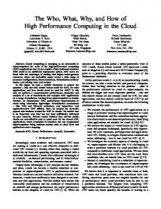
nodes can usually be added and removed during operation. The head node usually has two network interfaces, one to communicate with users outside of the cluster and another to communicate with the slave nodes. Hiding the slave nodes behind the front end allow for extra security and user authentication. Figure 1 illustrates a simple Beowulf cluster consisting of one master and two slave nodes.
Figure 1. A simple Beowulf Cluster consisting of one master and two slave nodes. The master node has two network interfaces to communicate with the slave nodes and users outside the cluster. Although clusters can be built using a variety of operating systems, LINUX is usually preferred. LINUX is open source and free so there is no “per node” licensing fees that could get expensive, especially with larger clusters. In addition, the open source environment allows users to make software changes, if necessary, to optimize the configuration. 2.
Primary Benefits
The primary benefits of clusters according to [4] are outlined below: •
Absolute scalability. It is possible to have dozens of machines, each of which is a multiprocessor. 4
•
Incremental scalability. The cluster is configured in such a way that it is possible to add new systems in small increments. Thus, a cluster can begin with a small system and increase its number of nodes without having to replace an older component with a newer one.
•
High availability. The failure of one node does not mean the loss of service unless the master node fails.
•
Superior price/performance. The cluster is constructed from commodity hardware. Therefore, a cluster can have equal or greater computing power than a single large machine at a lower cost.
3.
Cluster Classifications a.
Classification by Hardware
Clusters are most commonly classified by the hardware used to build it. Some clusters are built from components that can be found at your local computer store while others were specifically designed and built to be utilized in a cluster. Laptops can be used for experimental or instructive purposes. Often, desktop tower computers are stacked in rooms. Some computers such as blade servers are bought from a specific vendor and are intended for research or business. All of these computers have the ability to share peripherals with a keyboard video mouse (KVM) switch for configuration and trouble shooting purposes. b.
Classification by Network Technology
Clusters can also be classified by the type of network used to connect the nodes to one another. There are three common methods used to network clusters. (1) 10/100/1000 Base T Ethernet: The 1000 Mbps Ethernet is commonly referred to as Gigabit Ethernet. This is the most commonly used network technology in clusters and is also the network technology used in this thesis. It is
5
relatively inexpensive and has decent bandwidth. Although Ethernet’s latency is higher than that of Myrinet and Infiniband, it is still well suited for cluster computing. (2) Myrinet: Designed by Myricom [5], Myrinet is a high speed networking system with low overhead compared to Ethernet. This provides high throughput and less latency. Physically, Myrinet consists of two fiber optic cables (upstream and downstream) connected to the host with one connector. On the other end, machines are connected to low overhead routers and switches providing the connectivity. Myricom’s most recent network interface can reach speeds of up to 10-Gigabits per second. Myrinet is more expensive than Ethernet, but offers high bandwidth with low latency. (3) Infiniband: Infiniband [6] is a high performance, switched fabric interconnect standard for computers. Infiniband is designed for use in I/O networks such as data centers and clusters. Infiniband’s current limitation is 30 Gbps. Specifications for the Infiniband standard span multiple layers of the OSI model. The cost of Infiniband is also more than Ethernet, however high bandwidth is achieved with low latency. c.
Classification by Cluster Size
Clusters can be categorized from small to large based on the number of nodes.
d.
•
Mini cluster: 20 nodes
•
Midsize cluster: up to 50 nodes
•
Full cluster: more than 50 nodes Classification by Shared/No Shared Resources
According to Stallings [7], clusters can also be classified as to whether the individual nodes share access to the same disk. In a “no shared disk” configuration, each machine within the cluster has its own disk. In a “shared disk” configuration, the same 6
disk subsystem is connected to all the cluster’s nodes. Nodes using a “shared disk” configuration may also have their own disks installed. e.
Classification by Cluster Architecture
Another cluster classification, according to Stallings, is the distinction of separate servers, shared nothing, and shared disks. (1) Separate Servers: In separate servers, each node is a server with no shared disks among the servers. Although this offers high availability, it requires management or scheduling software to regulate traffic. If a node fails, another one will take over and complete the task. The availability is accomplished by copying data between the servers. The overhead of this constant data exchange ensures high availability but sacrifices the overall performance. The cluster implemented in this thesis is separate servers. (2) Shared Nothing: In order to reduce communication traffic, servers can be connected to common disks. This is “shared nothing.” The common disks can be partitioned where each node utilizes one volume. In the case of a node failure, another node will assume ownership of the volume and the cluster will continue to run. (3) Shared Disk: The third approach is called “shared disk.” With this configuration, multiple computers share the same disk at the same time so that each computer has access to all the volumes of the other computers. With this case, a locking mechanism is required to ensure that data on the disks can only be accessed by one process. 4.
Cluster Operating System
The operating system for a cluster must be specific for this special hardware configuration. Stallings [7] raises the following issues:
7
a.
Failure Management
There are two approaches that can be taken when dealing with failures: highly available clusters and fault tolerant clusters. If a failure occurs within a highly available cluster, another takes over. Any missing information as a result must be handled on the application level. A fault-tolerant cluster stores information on redundant shared disks that maintain the state of the system so that it can be easily retrieved in case of failure and continued. b.
Load Balancing
A cluster requires an effective ability for load balancing. Load-balancing clusters run by having all workload come through one or more load-balancing front ends. The front ends distribute the workload to a collection of back-end servers. c.
Parallelizing Computation
Clusters are built primarily to provide increased performance by dividing or splitting computational tasks across various nodes. Such clusters commonly run custom programs which have been designed to exploit the parallelism available. According to Kapp [8] there are three unique approaches to parallelizing applications. The software used in this thesis uses a combination of the first two. (1) Parallelizing Compiler: This approach at compile time determines the parts of an application that can be executed in parallel. These parts are then split off and assigned to various nodes. Performance can vary depending on the compiler. (2) Parallelized Application: From the beginning, the programmer builds the application so that it can be executed by the cluster and uses message passing to move data between nodes. Although this can make the programming more difficult, it increases the performance of the cluster. (3) Parametric Computing: This approach is used when the application involves an algorithm that must be performed numerous times, each time with 8
different input conditions. Extra organization and management tools are required for the separate jobs in order for this method to be effective. Parametric computing is usually implemented with a job scheduler, a system that allows the master node to distribute jobs to the slave nodes. B.
RELATED WORK Although there are numerous software packages available for parallel computing,
only implementations using Java are explored in this section. 1.
JavaParty
JavaParty provides a port for multi-threaded Java programs to distributed environments, like clusters [9].
It utilizes Java’s built in Remote Method Invocation
(RMI) library to communicate with the other nodes within the cluster. When writing Java code, the “remote” keyword is used to identify which objects are run remotely. The JavaParty compiler then generates the appropriate machine code needed to implement remote method invocations. JavaParty’s greatest advantage is that it significantly reduces the effort required to write a parallel Java program. 2.
Manta
Manta [10] is a native Java compiler that compiles Java source codes to x86 executables with a competitive goal to be faster than other current Java implementations, such as JavaParty. Although Manta uses a “highly efficient” RMI implementation, it does not have an efficient RMI package [11]. Manta supports the complete Java 1.1 language, including exceptions, garbage collection and dynamic class loading. Manta also supports some Java extensions, such as JavaParty’s “remote” keyword to identify remote classes. 3.
IceT
IceT [12] enables users to share Java Virtual Machines (JVMs) across a network. Users upload classes to other JVMs using a Parallel Virtual Machine (PVM) like interface. By explicitly calling send and receive statements, work can be distributed 9
among multiple JVMs. Fundamental to the IceT process model is the concept of process spoking, which refers to the ability of a process and its data to be uploaded to a remote computational resource for execution, as opposed to the common model of remote requests and responses. The main difference is that when a process is uploaded to a remote resource, it can exert independence from the requesting resource (unlike the RMI models), and can manage the uploading of any other processes that are necessary for the computation or to maintain persistent communications with other processes.
Like
JavaParty and Manta, IceT uses divide and conquer parallelism. 4.
mpiJava
The mpiJava distribution [13] is an object-oriented Java interface to the standard Message Passing Interface (MPI). It does this by providing Java wrappers, otherwise known as dummy classes, to a native MPI through the Java Native Interface. It does not assume any special extensions to the Java language. It is “portable” to any platform that provides compatible Java-development and native MPI environments.
10
III.
A.
JAVAPARTY
INTRODUCTION This chapter first presents a brief introduction to JavaParty’s communication
mechanism, RMI. Then, a brief explanation is presented regarding the transformation from “JavaParty code” to pure Java with RMI. Lastly, the Hello World example program is used to demonstrate how to write, compile, and run applications. B.
BACKGROUND RMI is a pure Java solution that allows applications to execute methods on remote
hosts such as servers or workstations. As the name suggests, it enables applications to locate and execute methods of a remote interface on a remote object. This process is transparent to the end user although remote hosts must have a Java Virtual machine installed. Most importantly, a method invocation on a remote object has the same syntax as a method invocation on a local object. 1.
Java RMI Architecture
Figure 2 illustrates the different layers of the Java RMI architecture. These layers are stubs and skeletons, remote reference layer, and transport layer.
Figure 2. a.
Java RMI Architecture
Stubs and Skeletons
RMI uses stubs and skeletons for communicating with remote objects. A stub for a remote object acts as a client's local representative or proxy for that object. 11
The caller invokes a method on the local stub which is responsible for carrying out the method call on the remote object. In RMI, a stub for a remote object implements the same set of remote interfaces that a remote object implements. When a stub’s method is invoked, it initiates a connection with the remote JVM containing the remote object and marshals (writes and transmits) the parameters. While the method is being invoked, the stub waits for the result. Once the stub receives the result, it unmarshals (reads) the return value or exception and then returns the value back to the caller. The stub makes the serialization parameters and the network-level communication transparent to the caller in order to present a simple invocation mechanism to the caller. For each remote object, there may be a skeleton in the remote JVM. The skeleton dispatches the call to the actual remote object implementation. When a skeleton first receives a method invocation it first unmarshals the parameters for the remote method. It then invokes the method on the actual remote object implementation before marshalling the result back to the caller. b.
Remote-Reference Layer
The remote-reference layer defines a RemoteRef interface. An implementation of this interface represents the link to the remote object and specifies the remote interaction’s call semantics. The stub stores a reference to a RemoteRef implementation and uses that object’s invoke() method to call remote methods. Changing the call semantics by using a nonstandard RemoteRef implementation is fully transparent to the client. c.
Transport Layer
The transport layer uses Java socket classes to handle communication between separate JVMs. Thanks to the socket-factory concept introduced in Java 1.2, the RMI system can use any stream-based communication.
12
2.
Threads
A thread is a software term that is short for “thread of execution.” They are a way for a program to split itself into two or more simultaneously running tasks. Many programs written today run as a single thread. This can cause problems when multiple events or actions need to occur simultaneously.
Multiple threads allow seamless
execution of two or more sections of a program at the same time. A method dispatched by the RMI runtime to a remote object implementation may or may not execute in a separate thread. The RMI runtime makes no guarantees with respect to mapping remote object invocations to threads. Since remote method invocation on the same remote object may execute concurrently, a remote object implementation needs to insure a thread-safe implementation. 3.
Garbage Collection
In Java, garbage collection deletes objects that are no longer referenced by a client. This eliminates the need for a programmer to keep track of the remote objects’ clients so that it can terminate.
RMI uses a reference-counting garbage collection
algorithm that keeps track of live references within each JVM. When a live reference enters a JVM, the count is increased; when it leaves it is decremented. After the last reference has been discarded, an unreferenced message is sent to the server. Sometimes a remote object is not referenced by any client. If this occurs, the RMI runtime refers to it with a weak reference. The weak reference enables the garbage collector to discard the object if no other local references exist. 4.
Class Loading
Parameters, return values, and exceptions passed in RMI calls are allowed to be any object that is serializable. RMI utilizes object serialization to send data to and from virtual machines. RMI also modifies the call stream with the proper location information allowing class definition files to be loaded at the receiver.
13
5.
Serialization
Serialization is the mechanism used by RMI to pass objects between JVMs, either as arguments in a method invocation from a client to a server or as return values from a method invocation. It involves saving the current state of an object to a stream, and restoring an equivalent object from that stream. The stream functions as a container for the object. Its contents include a partial representation of the internal structure of the object including variable types, names, and values. The container may be transient (RAM-based) or persistent (disk-based). A transient container may be used to prepare an object for transmission from one computer to another. A persistent container, such as a file on disk, allows storage of the object after the current session is finished. In both cases the information stored in the container can later be used to construct an equivalent object containing the same data as the original. 6.
Disadvantages of RMI
The first major disadvantage involves the language of RMI.
Program size
increases significantly when using RMI, making programming not only difficult, tedious and time-consuming, but also harder to manage [1]. For example, the classic program example, Hello World, is typically three to four lines of code using Java.
When
implementing the same code on remote machines using RMI, two sets of code are needed, one for the client and one for the server. Between both client and server codes, about 20 to 25 lines of code are necessary. The other major disadvantage is that RMI was designed for distributed programming and, therefore, is not really suited for parallel programming. RMI is too restrictive and the overhead for dealing with network problems is too verbose [1]. C.
THE JAVAPARTY PREPROCESSOR AND RUNTIME SYSTEM A multi-threaded Java program can be transformed into a distributed thread
JavaParty program with little effort and no increase in size [9]. This is done by identifying those classes and threads that can be run on another computer. These objects 14
are identified by using a class modifier called “remote”. This is the only extension of the language required. There is no need to map remote objects to a specific computer on the network. The compiler and runtime system assigns the objects to the various computers automatically. Objects that run locally are used locally without the cost of communication overhead. JavaParty is implemented as a pre-processing phase into Java compilers Espresso Grinder [14] and Pizza [15]. These compliers transform JavaParty code into pure Java with RMI hooks. The resulting code can then be compiled into machine code using a standard Java compiler. The JavaParty compiler, jpc, combines both steps so that JavaParty code is compiled right into machine code. This is illustrated in Figure 3.
Figure 3.
The JavaParty Compiler, JPC (From [1])
The runtime system consists of a main component called RuntimeManager and a subcomponent called LocalJP registered at the manager. A computer and its LocalJP can be added dynamically to the system. The manager knows the location of all LocalJPs and class objects. This allows the manger to know which computer implements the static part for each class that is loaded. This information is stored in all LocalJPs to reduce manager load.
Mangers and LocalJPs do not need to know the location of remote objects.
LocalJPs are used to call constructors in class objects and to implement both sides of a
15
migration. Figure 4 illustrates the relationships between the manager and the LocalJPs. Local JPs register with the manager to create remote objects and provide their current state when called.
Figure 4.
D.
JavaParty Runtime System (From [1])
RMI ENHANCEMETS WITH JAVAPARTY After JavaParty was created, its developers still were not fully satisfied with the
speed of RMI and serialization. Researchers developed a way to incorporate a more streamlined RMI called KaRMI. KaRMI improves the performance and flexibility of RMI. The basis behind KaRMI is to provide a lean and fast framework to plug in special purpose or optimized modules [11]. In addition, some enhancements were also made to the serialization process to improve its performance. 1.
RMI Improvements a.
Clean Interfaces between Design Layers
As with standard RMI design, KaRMI has three layers (stub/skeleton, reference, and transport). The outlining difference is that KaRMI has clear, distinct, documented interfaces between the layers [11]. This carries two advantages. 16
The first is that a remote method invocation only requires two additional method invocations at the interfaces between the layers and does not create temporary objects. This provides clean interfaces between layers. The second advantage is that alternative reference and transport implementations can be added with ease. This is contrary to RMI in that it exposes socket implementation to the application level. An example of this would be an application having the ability to export objects at specific port numbers. From their level, sockets belong to the transport layer. Making sockets visible at the application level means that RMI must use sockets at the transport layer. When sockets are used at this layer, the TCP/IP framework cannot be used and this slows down performance since datagram based transport layers are more efficient. The only way to fully take advantage of high speed networks is to separate Java’s sockets from the design of RMI. b.
Performance Improvements
Other performance improvements are summarized in [11] and are outlined below: •
For each remote method invocation KaRMI creates only a single object. This significantly improves performance over RMI that requires approximately 25 objects or more. Object creation in Java is expensive, so clean layering with fewer objects leads to improved performance.
•
The standard RMI uses costly calls of native code and the expensive reflection mechanism to find out about primitive types. There are two native calls per argument or non-void return value plus five native calls per remote method invocation. These can be avoided by a clever serialization. KaRMI uses native calls only for the interaction with device drivers.
•
In contrast to the official RMI, KaRMI's reference layer detects remote objects that happen to be local and short-cuts object access. 17
Of course, arguments will still be copied to retain RMI's remote object semantics. But, no thread switches and no communication are needed in KaRMI. •
The RMI designers prefer hash-tables over other data structures. Hash-tables are used where arrays would be faster or where KaRMI can avoid them completely. Although clearing hash-tables is slow, the RMI code frequently and unnecessarily clears hashtables before handing them to the garbage collector.
•
A little slowdown is caused on some platforms by the fact that the RMI code contains a lot of debugging code that is guarded by boolean ags (binary decision diagrams). At execution time, these ags are actively evaluated. KaRMI does not have any debugging code (instead we remove the debugging code by means of a preprocessor.)
c.
Pluggable Garbage Collection
Although RMI’s standard garbage collector is well designed to handle failures associated with wide-area networks, its tolerant features reduce efficiency [11]. When working with a closely connected cluster of computers, these features are not necessary and only inhibit performance.
KaRMI utilizes more efficient garbage
collectors designed for closely interconnect networks. 2.
Serialization Improvements a.
Reduced Type Information
Persistent objects must be readable after being stored to disk even if the byte array that was originally used to create the object is no longer obtainable. Because of this, Java’s method of serialization, or the functionality of writing and reading byte array representations, includes the complete type description in the stream of bytes representing an object being serialized. This is a drawback when using RMI for parallel computing 18
because this level of persistence is not required. The lifetime of an object is shorter than the runtime of the job. When objects are being sent, it is assumed that all nodes on the cluster have access to the same common file system. Therefore, encoding and sending the type information is unnecessary. JavaParty’s method of serialization improves performance by using textual encoding of class names and package prefixes to improve performance [11]. b.
Two Forms of Reset
To accomplish copy semantics, every new method must start with a clear hash-table. This enables objects that have already been transmitted to be re-transmitted with their current state. RMI can achieve this by creating a new JDK serialization object for each method invocation or by calling the serialization’s reset method.
The
disadvantage of both approaches is that both clear the information and types on objects already transmitted. UKA-serialization’s reset clears the objects hash table but leaves the type information untouched [11]. c.
Improved Buffering
JDK-serialization has two major drawbacks concerning buffering [11]. The first problem is that JDK-serialization uses buffered stream implementations on top of TCP/IP sockets that are general and lack information about object byte representation. With UKA-serialization, buffering is handled internally which allows byte information to be exploited. The second problem is that external buffering prevents programmers from directly writing into the buffers. With UKA-serialization, all necessary buffering is implemented itself. The buffer has also been made public so that marshaling routines can expedite their data directly into the buffer.
19
E.
WRITING, COMPILING, AND RUNNING APPLICATIONS 1.
Writing Applications a.
Extended JavaParty Syntax
As discussed, the JavaParty language extends Java with only one new modifier called remote. A class declaration can be prepended with this remote modifier to declare a class a remote class [9]. This is shown in the following sample code. public remote class R { /** instance variable of remote class */ public int x; /** instance method of remote class */ public void foo() { ... } /** static variable of remote class */ public static int y; /** static method of remote class */ public static void bar() { ... } }
The instances of a remote class are the "first class" members of a distributed JavaParty environment [9]. Even if they reside on different JVMs, they are able to interact with one another. In terms of syntax, there are no more differences between remote classes and non-remote classes.
Instances of remote classes are created with the remote
keyword, and the static and non-static members can be accessed just like they are in regular Java. Examples of instantiating and accessing a variable of a remote class are given as follows. // create an instance of remote class R R r = new R() // access an instance variable of the created remote object r.x = 42; // call its method foo() r.foo() // access a static member of the remote class R
20
R.y = 13; // call a static method of the remote class R.bar();
b.
Runtime System
The instance of operator in JavaParty is used to test whether an object is to be an instance of a certain class at runtime. Remote objects may be assigned to variables that are declared to be of type java.lang.Object [9]. This is illustrated in the following code. Object obj = new R(); // Test whether obj is an instance of remote class R. if (obj instanceof R) { ... }
2.
Setup
In order to compile and eventually run JavaParty applications, the JavaParty distribution must be downloaded and installed. Requirements, downloads and setup instructions are available from [9]. 3.
Compiling Applications
After JavaParty has been installed, Java applications written with JavaParty code can be compiled and tested. JavaParty programs can be compiled from any computer with Java SE 1.4.2 and of course JavaParty’s distribution installed. Note that JavaParty’s compiler is not yet compatible with Java SE 1.5 or above. To demonstrate the process, a rendition of Hello World called HelloJP provided by [9] will be used: package examples; public remote class HelloJP { public void hello() { // Print on the console of the virtual machine where the // object lives System.out.println("Hello JavaParty!"); }
21
public static void main(String[] args) { for (int n = 0; n < 10; n++) { // Create a remote object on some node HelloJP world = new HelloJP(); // Remotely invoke a method world.hello(); } } }
The following steps show how to compile HelloJP: 1.
Save the HelloJP source code to a file named HelloJP.java.
2.
Create a directory named classes where you wish to reside your
application classes to. mkdir classes
3.
Compile the program.
jpc -d classes HelloJP.java
4.
Running Applications
The following steps show how to run HelloJP: 1.
From the head node, set the class path (location of compiled classes). For
clusters without a distributed file system, a consistent copy of all the classes with the same path must be copied to each machine. setenv CLASSPATH classes
2.
Run the JavaParty application.
jpinvite examples.HelloJP
Remote objects are created on the virtual machines and the output message is printed on the head node’s console. Hello JavaParty!
22
IV.
A.
PERFORMANCE MEASUREMENTS
EXPERIMENTAL SETUP 1.
Hardware Configuration
The platform used was a cluster of eight servers. Four of the machines had AMD Opteron Dual-Core x86, 64-bit CPUs running at 2000 MHz. The hostnames of these machines were jp-1, jp-2, jp-3, jp-4. The other four had dual AMD Opteron Dual-Core x86, 64 bit processors running at 1600 MHz. The hostnames of these machines are jp-5, jp-6, jp-7 and jp-8.
All machines had 4 GB of RAM and 80 GB SATA hard disks.
Table 1 summarizes the above information. Figure 5, shown on the following page, is a photo of the cluster.
jp-1 to jp-4
jp-5 to jp-8
Type
Tyan
Tyan
CPU
2 GHz AMD Opteron Dual-Core Dual 2 GHz AMD Opteron Dual-Core x86, 64-bit (total two CPUs)
x86, 64-bit (total four CPUs)
Memory 4 GB
4 GB
HDD
80 GB
80 GB
NIC
Two (2) gigabit Ethernet network Two (2) gigabit Ethernet network adapters
adapters Table 1.
Hardware Configuration
The internal network switch was a Cisco Catalyst 3750 gigabit Ethernet switch. 2.
Operating System
Fedora Core 6 x86 64-bit was installed on all machines. Fedora Core is an open source LINUX distribution that does not require a license. Although JavaParty was 23
designed to work with the UNIX operating system, the LINUX command csh provides an enhanced but completely compatible version of the Berkeley UNIX C shell.
Figure 5. 3.
A photo of ECENET inside NPS’s High Performance Computing Center. Network Configuration
In order to connect the cluster to the NPS network, the following information below was provided by the NPS network administrator. This information was used to configure the external interface of the machine coordinating the parallelization of JVMs (head node or front end).
24
•
IP address and mask of the head node connected to the external network: This is 209.129.248.69 with mask 255.255.255.128. Note that in LINUX the network interface cards (NICs) are typically named eth0 for the internal (private) and eth1 for the external (public).
•
Domain name server IP addresses: This is 172.20.20.11 or 170.20.20.12.
•
Host name used for the head node: This is ecenet.hpr.nps.edu.
•
Local Gateway IP address: This is 209.129.248.1.
NICs in the machines belonging to the cluster were assigned IP addresses in the 5.1.1.0 network with mask 255.0.0.0. Figure 6 illustrates the cluster’s network configuration. The cluster is connected together with a gigabit switch and accessed via gateway 209.129.248.1 router. Table 2 provides a detailed look at the naming and addressing of hosts residing on the cluster’s internal network. For example, jp-5 has ip address 5.1.1.5 and subnet mask 255.0.0.0.
Figure 6.
The ECENET cluster (ecenet.hpr.nps.edu) with all the details. The host names of the nodes with the relevant IP addresses for the internal cluster along with the external network information are shown in the figure. 25
Hostname Alias Interface IP Address Mask ecenet.hpr.nps.edu jp-1 Private: eth0 5.1.1.1 255.255.255.0 Public: eth1 209.129.248.69 255.255.255.128 Jp-2 jp-2 eth0 5.1.1.2 255.0.0.0 Jp-3 jp-3 eth0 5.1.1.3 255.0.0.0 Jp-4 jp-4 eth0 5.1.1.4 255.0.0.0 Jp-5 jp-5 eth0 5.1.1.5 255.0.0.0 Jp-6 jp-6 eth0 5.1.1.6 255.0.0.0 Jp-7 jp-7 eth0 5.1.1.7 255.0.0.0 Jp-8 jp-8 eth0 5.1.1.8 255.0.0.0 Table 2. Node Naming and IP Addressing B.
BENCHMARKING Benchmarking is the process of characterizing the system as a whole or its various
subsystems in order to understand either its actual or potential performance. Benchmarking is used, generally speaking, for three purposes: measuring overall system performance in order to rank-order systems, measuring subsystem performance in order to make better optimization choices, and before-and-after comparisons to determine if changes have improved the performance of the system. A benchmark measures the ability of a machine to execute a series of tests. The results are usually recorded so that they can be used as a reference to be compared to other benchmark measurements. Each time an improvement or a change is made in the hardware and/or the software, the benchmarking can again be completed for comparison. Improvements are often compared to time and/or money spent to make the improvements. Although there are many open source benchmark programs available for clusters, most are designed for heterogeneous clusters utilizing an MPI. The JavaParty website [9] provides a handful of benchmarks which were all compiled and run. After examining some preliminary results, it was concluded that most of these benchmarks ran too quick to notice any significant improvements with the cluster. This was most likely due to the fact that these benchmarks were designed to run on machines from the late 90s. Despite
26
disappointment with not being able to utilize most of the benchmarks, one, named RayTracer, presented a more consistent, longer run time offering a more precise and accurate benchmark. Ray tracing is a technique used to model the path taken by light by following the rays of light as they interact with optical surfaces. The RayTracer benchmark creates a scene and then measures the performance of a 3D ray tracer.
The scene contains
numerous spheres rendered in high resolution. The outermost loop (over rows of pixels) has been parallelized using a cyclic distribution for load balance. After the program completes, the elapsed time is shown. The RayTracer JavaParty code was downloaded from [9]. It was then compiled using jpc and run using jpinvite. Figure 7 is a screenshot of the terminal window running the RayTracer benchmark.
Figure 7.
RayTracer Benchmark Screenshot 27
The test was run 50 consecutive times with two machines, three machines, four machines, six machines and eight machines. The mean and standard deviation of the elapsed time for each set was computed. The results are summarized in Table 3 and are shown in Figure 8. It is apparent from these results that the speed-up of RayTracer is relative to the number of machines included in the execution. Comparing the mean execution times, adding two more machines to the original two decreased the execution time significantly from 73.79 seconds to 50.78 seconds. Adding six machines to the original two (total eight machines) decreased the run time to 21.45 seconds.
Number of Machines 2 3 4 6 8 Mean elapsed time (sec) 73.79 50.78 38.10 27.12 21.45 Σ 29.09 18.08 8.82 6.01 3.28 Table 3. RayTracer Benchmark Results Summary
Mean Elapsed Time vs Number of Machines
mean elapsed time (sec)
80 70 60 50 40 30 20 10 0 0
1
2
3
4
5
6
7
8
9
number of machines Mean Elasped Time
Figure 8.
Standard Deviation
Execution Times for RayTracer Benchmark
While running the experiment, it was noticed that some of the CPUs configured to run did not always run. For example, if jp-1 and jp-2 were configured to run RayTracer, occasionally only jp-1’s CPU would partake in the execution of the program. Due to this 28
occurrence, the standard deviation was higher than expected, especially for the execution times using fewer machines. Although the specific reasons why this happened go beyond this thesis, a request to the developers of JavaParty was made to provide a brief answer and no response was received.
29
THIS PAGE INTENTIONALLY LEFT BLANK
30
V.
A.
OPTIMIZING CLUSTER PERFORMANCE
INTRODUCTION It is now apparent that running Java applications using multiple virtual machines
provides a significant time advantage to the user. Many users, however, may not have access to a cluster on a congestion-free network. This chapter attempts to evaluate the performance of the cluster running the same RayTracer benchmark, only this time with network congestion.
In addition, an attempt is made to prioritize JavaParty’s network
traffic using a Cisco Catalyst 3750 Ethernet switch to improve the benchmark mean execution run time. B.
JAVA PARTY TRAFFIC ANALYSIS In order to understand and remedy the negative impact of network congestion, it
is first important to have a thorough understanding of the different traffic types and flow patterns associated with JavaParty’s communication mechanism. To do this, the network protocol analyzer Ethereal was utilized. Two ports on the Cisco Catalyst 3750 Ethernet switch were configured to replicate the ports connecting jp-1 and jp-2. While running the RayTracer benchmark, network traffic flowing in and out of jp-1 and jp-2 was simultaneously captured using Ethereal. From the data capture, the protocols and flow patterns were examined. From the transport layer perspective, all traffic generated by the JavaParty runtime system was Transmission Control Protocol (TCP). Using TCP guarantees that all JavaParty traffic moving within the cluster’s internal network reaches its destination in the correct order with no errors. Ethereal identified five types of TCP traffic: low level control/acknowledgment (control/ACK), Secure Shell (SSH), short frame, data, and RMI. Control/ACK traffic is used to ensure proper packet delivery. SHH is an application layer protocol “on top” of TCP that allows data to be exchanged securely between two computers. Packets 31
identified as short frame, or truncated (Ethereal often truncates large packets), are usually for carrying large amounts of data. Along with most short frame packets, data packets are also used to transport data. The Java RMI protocol is the Java technology-specific protocol for looking up and referencing remote objects. Like SSH, it is an application level protocol running under the RMI layer and over TCP. From the data capture, statistics were collected regarding each type of traffic. Figure 9 illustrates the percentage of each type of packet captured. The majority were Control/ACK and SSH packets. There were only 15 RMI packets captured. Number of Packets Data 18,416
RMI 15
Short Frame 27,020
Control/ACK 65,664
SSH 61,226
Figure 9.
Number of packets for one execution of RayTracer using 4 hosts.
Figure 10 graphs mean packet length for each traffic type. From the graph it is seen that control/ACK packets are smaller in size and short frame and data packets are larger. Control/ACK packets are smaller because they are not carrying actual data. Data packets attempt to maximize data transfer with as little overhead as possible.
32
Mean Packet Length 1230 1049
Length (bytes)
1030
965
830 630 430
336
230
138
66 30 Control/ACK Figure 10.
SSH
Short Frame
Data
RMI
Mean packet length for one execution of RayTracer using 4 hosts.
To understand how the JavaParty runtime system loads the cluster’s internal network, a running average of the bit rates for each type of JavaParty traffic was plotted. Data used to create the first set of plots (Figures 11 through 14) was captured from the jp1’s Ethernet port during an execution of RayTracer using four hosts. This data comprises traffic moving to and from the head node to all other nodes in the cluster. The second set of plots (Figures 15 through 18) used data captured from jp-2’s Ethernet port. This data represents data moving to and from a slave node. Due to the relatively small number of RMI packets in the capture, the RMI plots are not shown. Figures 11 and 15 show low level control/ACK traffic for both the head and slave nodes. The relatively lower but consistent bit rates plotted are reflective of typical control/ACK traffic. Due to smaller packet sizes, bit rates are lower while the flow is consistent due to continuous traffic control. For similar reasons SSH traffic, shown in Figures 12 and 16, has a similar plot to control/ACK traffic except these packets are encrypting rather than controlling. 33
Data flow can be observed in Figures 13, 14, 17, and 18. Although the short frame traffic remains consistent, spikes in data traffic can be observed. Similar but smaller spikes can be observed in the control/ACK and SSH packets. These small spikes show that extra control/ACK and SSH packets are needed during times of increased data flow.
Figure 11.
Plot of head node low level control/ACK bit rate for one execution of RayTracer using four hosts.
34
Head Node SSH Bit Rate 300
data rate (Mbps)
250 200 150 100 50 0 0
5
10
15
20
25
30
35
40
time (sec)
Figure 12.
Plot of head node SSH bit rate for one execution of RayTracer using four hosts.
Head Node Short Frame Bit Rate 300
data rate (Mbps)
250 200 150 100 50 0 0
5
10
15
20
25
30
35
40
time (sec)
Figure 13.
Plot of head node short frame bit rate for one execution of RayTracer using four hosts. 35
Head Node Data Bit Rate 300
data rate (Mbps)
250 200 150 100 50 0 0
5
10
15
20
25
30
35
40
time (sec)
Figure 14.
Plot of head node data bit rate for one execution of RayTracer using four hosts. Slave Node Low Level Control/ACK Bit Rate
300
data rate (Mbs)
250 200 150 100 50 0 0
5
10
15
20
25
30
35
40
time (sec)
Figure 15.
Plot of slave node low level control/ACK bit rate for one execution of RayTracer using four hosts. 36
Slave Node SSH Bit Rate 300
data rate (Mbps)
250 200 150 100 50 0 0
5
10
15
20
25
30
35
40
time (sec)
Figure 16.
Plot of slave node SSH bit rate for one execution of RayTracer using four hosts. Slave Node Short Frame Bit Rate
300
data rate (Mbps)
250 200 150 100 50 0 0
5
10
15
20
25
30
35
40
time (sec)
Figure 17.
Plot of slave node short frame bit rate for one execution of RayTracer using four hosts.
37
Slave Node Data Bit Rate 300
Data Rate (Mbps)
250 200 150 100 50 0 0
5
10
15
20
25
30
35
40
time (sec)
Figure 18.
C.
Plot of slave node data bit rate for one execution of RayTracer using four hosts.
OPTIMIZING JAVA PARTY IN A CONGESTED NETWORK 1.
Congesting the Network
In order to evaluate how JavaParty applications respond to a congested network, congestion was simulated by bombarding each machine with User Datagram Protocol (UDP) packets. UDP was used because it is a core protocol of the Internet Protocol (IP) suite and it does not guarantee arrival or ordering like, for example, TCP. This insured that each trial was similar in that extra traffic was not generated due to the randomness of lost packets or collisions. Because half of the machines were needed to generate the congestion, the experiments in this segment were limited to four machines. The experiment was performed so that the machines running RayTracer (jp-1, jp-2, jp-3 and jp-4) were simultaneously bombarded with UDP packets by jp-5, jp-6, jp-7 and jp-8 respectively. The traffic was generated using a program called D-ITG 2.4 [16]. To keep the traffic at a 38
consistent rate, a constant packet inter-departure time was configured. In addition, the packets were sent at the maximum inter-departure rate and maximum size (1400 Byte payload). Figure 19 shows a screen capture of the D-ITG packet generator software configured to bombard jp-1 (5.1.1.1).
Figure 19.
The D-ITG GUI configured to bombard jp-1 (5.1.1.1).
RayTracer was run again 50 consecutive times using four machines, this time with congestion. The results are shown in Table 4. The average time it took to run the benchmark was dramatically slower compared to the first trial done without congestion. After adding congestion, the RayTracer benchmark takes on average an additional 19.8 seconds to run. The cause of the slowdown in most likely due to the following: •
First in first out (FIFO) priority on all packets (including UDP packets)
•
Buffers on the switch reaching capacity and dropping packets
•
Decreased CPU availability on machines due to handling of incoming UDP packets
The standard deviation also increased indicating individual trials were wider spread and varied more from the mean. 39
No congestion With congestion Difference Mean elapsed time (sec) 38.10 57.90 19.8 Σ 8.82 11.83 3.01 Table 4. RayTracer benchmark results using 4 machines. Execution times are slower with generated congestion 2.
Improving Cluster Performance with QoS
In some cases avoiding network congestion may be inevitable, and as it was shown in the previous section, it can significantly hinder performance. One example of this type of situation is a LINUX cluster interconnected with a network that is also utilized by other users. Cisco advertises that the Catalyst 3750 switch offers features and benefits that can increase performance in congested LINUX cluster environments [17]. In this section, the capabilities of the switch are determined and applied with an objective to improve the mean execution time of RayTracer with network congestion. Typically, networks run on the best-effort, FIFO delivery basis. This means that all network traffic has equal priority with an equal chance of being dropped. The Cisco Catalyst 3750 has the capability to police and prioritize traffic using QoS (Quality of Service). To implement QoS, the switch classifies the network traffic according to a profile created by the user. Incoming traffic to the switch can be classified with a CoS (Class of service) value in the ISL/802.1Q/802.1p frame (Layer 2) or with an IP precedence or DSCP (Differentiated Services Code Point) in the ToS (Type of Service) field located in the IP packet header (Layer 3). CoS and IP precedence values range from zero to seven, seven being the highest priority. DSCP values range from zero to 63, 63 being the highest priority. Figure 20 illustrates QoS classification layers in frame and packets. For example, three bits are used for CoS in the ISL (Inter-Switch Link) frame and one byte of IP precedence is used for the IPv4 packet.
40
Figure 20.
QoS Classification layers in frames and packets (From [2])
After the packets have been classified, they are policed to determine whether they are in or out of profile. A policer has the ability to adjust bandwidth consumed by traffic before passing the result to the marker. The marker considers information passed by the policer and the QoS profile in making the decision on what to do with the packet. The marker can either drop the packet or allow it to pass through to the ingress queues. During this decision, the marker also modifies the contents of the CoS and ToS values inside the frame or packet header in accordance with the QoS profile. Once the packet arrives at the ingress queue, queuing and scheduling moves the packet through the remainder of the switch. Figure 21 illustrates this process in a basic QoS model. It is divided into two sections, actions at ingress for incoming packets and actions at egress for outgoing packets.
41
Figure 21.
Basic QoS Model (From [2])
The Catalyst 3750 has two ingress queues that queue packets for entry. The QoS profile can specify the specific queue to handle packets of different Cos or ToS values. The two ingress queues are outfitted with a weighted tail-drop (WTD) algorithm to avoid congestion. When the threshold for a particular class of packet specified is exceeded, the packets are dropped. The switch’s scheduling mechanism services the queues based on shaped round robin (SRR) weights also specified in the QoS profile. The SRR weights determine the frequency at which the switch services the ingress queues. In addition, one of the ingress queues is considered the priority queue. SRR services the priority queue for its configured share before servicing the other queue. Similarly, when a packet arrives at the egress queue, the packet’s QoS label and CoS value decide which egress queue out of the four will be used. The egress queues use the same WTD and SRR weight concepts as the ingress queues in determining packet drops and scheduling. The first egress queue (Queue 1) can be configured as the expedited queue. This queue is emptied before the other queues are serviced. 3.
Configuring QoS a.
Classifying Traffic
With a clear understanding of JavaParty’s protocols and flow patterns, the decisions involved with classifying the traffic became trivial: assign JavaParty traffic a higher priority than the generated traffic causing the congestion. To implement this idea, 42
a method was needed to isolate JavaParty traffic from as much other traffic as possible. The Catalyst 3750 offers a number of ways of doing this. Packets can be classified solely by host, destination, or IP protocol type or any combination of these three unique identifiers. Since all JavaParty traffic is TCP and only exists between JP-1, JP-2, JP-3 and JP-4, a policy was created that changed the DSCP value of each IP header to 40 given this occurrence. It would have been preferred to further prioritize the JavaParty TCP traffic at the application level. However, since the switch is only able to prioritize traffic at the transport layer, this could not be done. All other packets defaulted to DSCP value 0 (routine traffic). b.
Queuing and Scheduling Configuration
Since there are two ingress queues on the Catalyst 3750 (Queue 2 being priority), it was again trivial to send JavaParty traffic through Queue 2. Queue two was configured to handle DSCP levels 40-47. If JavaParty traffic and routine traffic used the same queue, WTD thresholds could be set to keep the JavaParty traffic and drop the routine traffic overloading the queue. Because JavaParty traffic uses an entirely different queue than routine traffic, there was no need to configure special WTD thresholds. Since Queue 1 was handling the majority of traffic, 85% of the buffer space was allocated to it. By default, this left a generous 15% of the buffer space bandwidth to Queue 2 handling solely JavaParty traffic. In addition, SRR bandwidth weights were configured to allocate Queue 2 the maximum amount of bandwidth available when JavaParty traffic was present. This was done by setting Queue 2 as the priority queue which guaranteed bandwidth in the presence of congestion. A similar configuration was setup on the four egress queues. Queue 1 was configured to accept packets only with DSCP 40-47. A generous 15% of the buffer space was allocated to Queue 1 handling JavaParty traffic and 65% to Queue 2 handling the routine traffic. The rest of the buffer space was split evenly between the last two queues. Just like the ingress queues, the egress queue’s SRR bandwidth weights were configured to allocate Queue 1 the maximum amount of bandwidth available when JavaParty traffic 43
was present. In addition, Queue 1 was configured as the expedite queue. The expedite queue is serviced and emptied before servicing any other queue. 4.
RayTracer Revisited
To test the QoS profile created for the cluster, RayTracer with four hosts was used again as a Benchmark. To ensure that the profile was not hindering the cluster’s performance, the benchmark was run with the QoS profile and no congestion so it could be compared to the mean execution time with no profile and no congestion. The mean runtime increased slightly to 40.05 seconds, a 1.95 second increase. Since the standard deviation was high for the execution times revealed in the previous chapter, this increase is not significant enough to associate the slow down with the profile. With the QoS profile still in place, RayTracer was run another 50 times with added network congestion. The profile decreased the execution time from 57.90 seconds to 44.07 seconds, a significant decrease in time. With no network congestion, the mean run time with the QoS profile was only 1.95 seconds from the mean run time with no QoS profile. When network congestion was added, the QoS improved RayTracer’s mean execution time by 13.83 seconds, a significant and notable improvement. The results are summarized in Table 5 and shown in Figure 22.
No With No With congestion, congestion, congestion, congestion, No QoS No QoS w/ QoS w/ QoS Mean elapsed time (sec) 38.10 57.90 40.05 44.07 Σ 8.82 11.83 9.37 8.91 Table 5. RayTracer benchmark results using four machines and a QoS profile. The QoS profile significantly decreases the RayTracer mean runtime in the presence of generated network congestion.
44
Mean Execution Times 60.00
mean runtime (sec)
55.00 50.00 45.00 40.00 35.00 30.00
No Congestion, No QoS
Congestion, No QoS
No Congestion, w/ QoS
Congestion, w/ QoS
Figure 22. A comparison of RayTracer execution times under different testing conditions. The chart illustrates the time lost due to network congestion, and how the QoS profile prioritized cluster traffic to reduce execution time.
45
THIS PAGE INTENTIONALLY LEFT BLANK
46
VI. A.
CONCLUSIONS AND FUTURE WORK
CONCLUSIONS The research completed in this thesis showed that when implementing a parallel
Java system using JavaParty, faster program execution times can be achieved by adding additional JVMs. In the presence of network congestion, a QoS profile can be configured with the cluster interconnect to prioritize JavaParty traffic between the nodes significantly increasing performance. This research also verified that JavaParty is truly an elegant way to implement a cluster with Java. The code of JavaParty parallel programs are significantly shorter and less complex than RMI based parallel programs making them easier to work with. Also compared to traditional RMI, JavaParty programs also adapt more flexibly to various network conditions and can exploit locality. JavaParty’s enhanced runtime system and serialization is faster and more efficient compared with Java’s standard environment providing a more suited service for a closely connected cluster. Finally, this research delivered a “product” to the advanced networking laboratory that provides a less tedious method and a more powerful platform to parallelize and run Java applications. To comment on building the cluster, implementation required significant LINUX and UNIX expertise. Anyone setting up a LINUX cluster should also be familiar with the accompanying tools and utilities of the LINUX OS. It is difficult for a person not experienced in UNIX to accomplish a completely correct installation. Solutions for problems are not always instantly available and time has to be spent searching several resources. The manuals do not cover all possible problems. B.
FUTURE WORK As described in the related work portion of this thesis, there are other alternatives
to implementing fast parallel Java that may be faster then JavaParty. Some of these options may be worth exploring although JavaParty seems to be an efficient choice when considering the investment of time spent programming. The trade-off lies between cluster performance and ease of programming. 47
For now, the cluster is configured and ready to run parallel JavaParty applications. The advanced networking laboratory plans on using the cluster for network protocol simulation and research concerning mobile ADHOC and sensor networks. Having the cluster available as a tool will significantly improve research productivity.
48
APPENDIX A
Recorded RayTracer execution times for the various configurations discussed are included in this appendix. 1.
RayTracer Execution Times (From Chapter IV)
The following table includes the data obtained by running RayTracer. The first column shows the times when only two hosts were used. The next column includes three hosts, and etcetera. Trial # 1 2 3 4 5 6 7 8 9 10 11 12 13 14 15 16 17 18 19 20 21 22 23 24 25 26 27 28 29 30 31 32 33
jp-1 – 2 95.35 123.48 47.94 85.39 94.74 102.41 48.86 50.65 45.62 93.77 96.92 48.99 124.22 47.27 47.45 96.24 45.69 49.93 47.11 86.96 48.11 122.87 48.63 45.11 122.01 46.36 121.40 50.38 45.19 46.87 88.21 104.56 47.36
jp-1 -3 44.10 34.83 50.96 49.52 34.91 48.11 49.39 44.80 32.62 91.25 44.98 46.14 45.94 94.31 50.17 51.05 48.40 32.90 48.69 33.90 46.81 46.91 46.31 50.20 91.09 45.80 47.21 50.00 46.15 50.37 34.02 33.63 32.57
jp-1 - 4 33.87 32.29 32.29 30.76 44.23 44.78 49.33 35.55 32.85 33.41 47.54 33.60 51.02 50.53 52.17 31.72 33.83 46.17 25.08 32.62 47.51 33.93 33.03 34.46 32.09 30.86 25.98 54.97 49.35 30.48 48.14 33.70 55.31
49
jp-1 - 6 24.15 20.74 21.62 26.28 20.99 21.36 34.17 33.79 27.16 22.90 35.30 27.38 22.36 26.00 21.41 27.17 25.78 28.86 21.30 26.39 21.35 27.69 27.33 18.57 26.10 33.12 21.56 34.33 33.45 28.33 26.83 25.63 36.33
jp-1 -8 22.63 16.30 18.62 19.53 19.38 16.75 18.37 20.07 25.64 18.45 18.80 17.98 23.63 27.13 22.46 24.62 17.96 23.30 27.01 22.38 25.18 24.69 15.65 26.43 23.73 25.36 24.52 22.37 16.24 17.71 20.75 19.45 22.11
34 35 36 37 38 39 40 41 42 43 44 45 46 47 48 49 50 Avg σ
2.
92.92 107.60 48.28 49.14 45.97 49.80 50.06 52.65 95.07 125.67 51.39 88.98 49.09 111.95 88.81 92.04 73.79 29.09
49.07 45.56 33.06 45.90 46.16 48.72 49.05 48.36 50.52 47.66 50.16 124.70 48.08 52.31 56.18 98.59 46.95 50.78 18.08
44.46 33.34 32.50 33.21 34.88 33.21 25.65 31.98 48.33 25.15 32.40 53.97 31.91 33.33 35.10 57.93 34.30 38.10 8.82
26.83 26.02 23.86 34.91 27.07 22.18 17.69 25.84 26.65 52.48 33.80 26.64 20.53 28.22 25.51 35.11 26.93 27.12 6.01
19.27 18.19 25.44 24.46 20.90 18.58 25.73 20.44 21.19 22.46 21.74 17.43 21.65 28.59 17.91 21.29 21.95 21.45 3.28
RayTracer Execution Times (From Chapter V)
The first set of data is with the QoS profile enabled but with no generated traffic. The second case is with generated traffic but no QoS profile. The third case is with QoS enabled with generated traffic. Trial # 1 2 3 4 5 6 7 8 9 10 11 12 13 14 15 16 17 18
w/ QoS, no traffic 37.49 50.85 38.48 49.62 47.37 38.88 33.58 25.00 43.53 38.72 32.63 38.34 32.92 60.19 45.92 45.86 46.28 54.38
No QoS, w/ traffic 72.76 56.89 60.45 56.35 60.79 69.32 59.97 52.78 76.23 64.88 44.86 49.93 82.22 52.95 62.86 48.68 70.56 57.32
50
w/ QoS, w/ traffic 34.82 37.13 56.60 30.82 56.50 40.25 37.62 46.37 43.79 36.74 46.57 50.56 48.92 62.28 43.65 50.92 39.40 32.31
19 20 21 22 23 24 25 26 27 28 29 30 31 32 33 34 35 36 37 38 39 40 41 42 43 44 45 46 47 48 49 50 Avg σ
37.40 34.65 40.41 26.47 48.11 25.41 26.12 50.26 33.88 32.38 51.66 37.25 34.68 36.25 37.00 32.65 46.38 46.83 33.04 31.37 59.23 37.75 43.32 33.55 33.29 60.59 49.58 29.74 25.52 31.48 51.03 44.99 40.05 9.37
76.01 50.64 44.58 42.31 66.25 41.63 45.20 72.42 64.16 58.88 59.23 58.49 49.15 48.91 59.83 43.18 42.45 34.52 67.74 55.94 63.62 45.32 34.19 54.20 44.64 79.94 54.12 75.10 59.81 64.87 87.82 50.28 57.90 11.83
51
57.07 52.48 36.79 48.85 51.92 47.92 54.11 62.35 37.70 29.20 42.60 29.69 39.03 49.22 37.33 45.42 45.24 36.48 39.72 37.14 56.67 42.10 63.34 46.85 50.76 37.68 43.99 47.49 30.48 34.53 38.45 35.42 44.07 8.91
THIS PAGE INTENTIONALLY LEFT BLANK
52
APPENDIX B
This appendix includes the QoS configuration of the Cisco Catalyst 3750 switch used to improve cluster performance with generated traffic. 1.
Cisco Catalyst 3750 Running Configuration
Switch#show access-lists Current configuration : 4691 bytes ! version 12.1 no service pad service timestamps debug uptime service timestamps log uptime no service password-encryption ! hostname Switch ! ! ip subnet-zero ! mls qos srr-queue input bandwidth 1 99 mls qos srr-queue input buffers 70 30 mls qos srr-queue input priority-queue input 2 bandwidth 40 mls qos queue-set output 2 threshold 1 400 400 100 400 mls qos queue-set output 2 threshold 2 40 60 100 200 mls qos queue-set output 2 buffers 50 40 5 5 mls qos ! class-map match-all class134 match access-group 134 class-map match-all class143 match access-group 143 class-map match-all class124 match access-group 124 class-map match-all class142 match access-group 142 class-map match-all class114 match access-group 114 class-map match-all class141 match access-group 141 class-map match-all class112 match access-group 112 class-map match-all class121 match access-group 121 class-map match-all class113 match access-group 113 class-map match-all class131 match access-group 131 class-map match-all class123 match access-group 123
53
class-map match-all class132 match access-group 132 ! ! policy-map police-jp class class112 set ip dscp 40 class class113 set ip dscp 40 class class114 set ip dscp 40 class class121 set ip dscp 40 class class123 set ip dscp 40 class class124 set ip dscp 40 class class131 set ip dscp 40 class class132 set ip dscp 40 class class134 set ip dscp 40 class class141 set ip dscp 40 class class142 set ip dscp 40 class class143 set ip dscp 40 ! ! spanning-tree mode pvst no spanning-tree optimize bpdu transmission spanning-tree extend system-id ! ! interface GigabitEthernet1/0/1 no ip address srr-queue bandwidth share 97 1 1 1 queue-set 2 priority-queue out service-policy input police-jp no mdix auto ! interface GigabitEthernet1/0/1.24 srr-queue bandwidth share 97 1 1 1 queue-set 2 priority-queue out ! interface GigabitEthernet1/0/2 no ip address srr-queue bandwidth share 97 1 1 1 queue-set 2 priority-queue out service-policy input police-jp
54
no mdix auto ! interface GigabitEthernet1/0/3 no ip address srr-queue bandwidth share 97 1 1 1 queue-set 2 priority-queue out service-policy input police-jp no mdix auto ! interface GigabitEthernet1/0/4 no ip address srr-queue bandwidth share 97 1 1 1 queue-set 2 priority-queue out service-policy input police-jp no mdix auto ! interface GigabitEthernet1/0/5 no ip address no mdix auto ! interface GigabitEthernet1/0/6 no ip address no mdix auto ! interface GigabitEthernet1/0/7 no ip address no mdix auto ! interface GigabitEthernet1/0/8 no ip address no mdix auto ! interface GigabitEthernet1/0/9 no ip address no mdix auto ! . . . . . ! interface Vlan1 no ip address shutdown ! ip classless ip http server ! access-list 100 permit ip any any access-list 112 permit ip host 5.1.1.1 host 5.1.1.2 access-list 113 permit ip host 5.1.1.1 host 5.1.1.3 access-list 114 permit ip host 5.1.1.1 host 5.1.1.4
55
access-list 121 access-list 123 access-list 124 access-list 131 access-list 132 access-list 134 access-list 141 access-list 142 access-list 143 ! line con 0 line vty 5 15 ! ! monitor session monitor session monitor session monitor session
permit permit permit permit permit permit permit permit permit
1 1 2 2
ip ip ip ip ip ip ip ip ip
host host host host host host host host host
5.1.1.2 5.1.1.2 5.1.1.2 5.1.1.3 5.1.1.3 5.1.1.3 5.1.1.4 5.1.1.4 5.1.1.4
host host host host host host host host host
source interface Gi1/0/1 destination interface Gi1/0/21 encapsulation replicate source interface Gi1/0/2 destination interface Gi1/0/22 encapsulation replicate
end 2.
QoS Access Lists
Switch#show access-lists Extended IP access list 100 permit ip any any Extended IP access list 112 permit ip host 5.1.1.1 host Extended IP access list 113 permit ip host 5.1.1.1 host Extended IP access list 114 permit ip host 5.1.1.1 host Extended IP access list 121 permit ip host 5.1.1.2 host Extended IP access list 123 permit ip host 5.1.1.2 host Extended IP access list 124 permit ip host 5.1.1.2 host Extended IP access list 131 permit ip host 5.1.1.3 host Extended IP access list 132 permit ip host 5.1.1.3 host Extended IP access list 134 permit ip host 5.1.1.3 host Extended IP access list 141 permit ip host 5.1.1.4 host Extended IP access list 142 permit ip host 5.1.1.4 host Extended IP access list 143 permit ip host 5.1.1.4 host
3.
5.1.1.1 5.1.1.3 5.1.1.4 5.1.1.1 5.1.1.2 5.1.1.4 5.1.1.1 5.1.1.2 5.1.1.3
5.1.1.2 5.1.1.3 5.1.1.4 5.1.1.1 5.1.1.3 5.1.1.4 5.1.1.1 5.1.1.2 5.1.1.4 5.1.1.1 5.1.1.2 5.1.1.3
QoS Class Maps
Switch#show class-map
56
Class Map match-any class-default (id 0) Match any Class Map match-all class134 (id 10) Match access-group 134 Class Map match-all class143 (id 13) Match access-group 143 Class Map match-all class124 (id 7) Match access-group 124 Class Map match-all class142 (id 12) Match access-group 142 Class Map match-all class114 (id 4) Match access-group 114 Class Map match-all class141 (id 11) Match access-group 141 Class Map match-all class112 (id 2) Match access-group 112 Class Map match-all class121 (id 5) Match access-group 121 Class Map match-all class113 (id 3) Match access-group 113 Class Map match-all class131 (id 8) Match access-group 131 Class Map match-all class123 (id 6) Match access-group 123 Class Map match-all class132 (id 9) Match access-group 132
4.
QoS Policy Maps
Switch>show policy-map Policy Map police-jp class class112 set ip dscp 40 class class113 set ip dscp 40 class class114 set ip dscp 40 class class121 set ip dscp 40 class class123 set ip dscp 40 class class124 set ip dscp 40 class class131
57
set ip dscp 40 class class132 set ip dscp 40 class class134 set ip dscp 40 class class141 set ip dscp 40 class class142 set ip dscp 40 class class143 set ip dscp 40
58
LIST OF REFERENCES [1]
M. Philippsen and M. Zenger, “JavaParty: Transparent Remote Objects in Java,” IEEE Concurrency, Vol. 9, No. 11, pp.1125-1242, 1997.
[2]
Cisco, "Catalyst 3750 Switch Software Configuration Guide, 12.2(25)SEE," p. 1, 2007.
[3]
Beowulf.org. Retrieved Feb 11, 2007 from http://www.beowulf.org.
[4]
E. Brewer, "Clustering: Multiply and Conquer," Data Communications, July 1997.
[5]
Myricom Inc. Retrieved February 7, 2007 from http://www.myri.com.
[6]
Infiniband Trade Association. Retrieved February 7, 2007 from http://www.infinibandta.org/home.
[7]
W. Stallings, Operating Systems. 4th ed., Upper Saddle River: Prentice Hall, 2001, p. 779.
[8]
C. Kapp, “Managing Cluster Computers,” Dr. Dobb’s Journal, July 2000.
[9]
JavaParty. Retrieved May 4, 2007 from http://svn.ipd.unikarlsruhe.de/trac/javaparty.
[10]
Manta: Fast parallel java. Retrieved May 20, 2007 from www.cs.vu.nl/manta.
[11]
B. Haumacher, M. Philippsen, and C. Nester. A More Efficient RMI for Java. Concurrency: Practice and Experience, 12(7):495-518, May 2000.
[12]
P. Gray and V. S. Sunderam. IceT: Distributed Computing and Java. Retrieved May 9, 2007 from http://citeseer.ist.psu.edu/192886.html.
[13]
mpiJava. Retrieved May 14, 2007 from http://www.npac.syr.edu/projects/pcrc/mpiJava/mpiJava.html.
[14]
M. Odersky and M. Philippsen. Espresso Grinder. Retrieved May 7, 2007 from http://www.ipd.ira.uka.de/~espresso.
[15]
M. Odersky and P. Wadler. Pizza into Java: Translating theory into practice. In Proc. 24th ACM Symposium on Principles of Programming Languages, January 1997. 59
[16]
Distributed Internet Traffic Generator. Retrieved on May 9, 2007 from http://www.grid.unina.it/software/ITG.
[17]
Cisco. Using the Cisco Catalyst 3750 Series Switch as a Gigabit Linux Cluster Interconnect. p. 1, 2003.
60
INITIAL DISTRIBUTION LIST 1.
Defense Technical Information Center Ft. Belvoir, Virginia
2.
Dudley Knox Library Naval Postgraduate School Monterey, California
3.
Professor Jeffrey Knorr Department of Electrical and Computer Engineering Naval Postgraduate School Monterey, California
4.
Professor Weilian Su Department of Electrical and Computer Engineering Naval Postgraduate School Monterey, California
5.
Mr. Bob Broadston Naval Postgraduate School Monterey, California
61


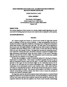


![Java in High-Performance Computing - GeeCON [PDF]](https://m.moam.info/img/260x300/java-in-high-performance-computing-geecon-pdf_6479c803098a9e02488b456c.jpg)