High-Performance Quantum Computing Simulation for the Quantum ...

High-Performance Quantum Computing Simulation for the Quantum Geometric Machine Model Adriano Maron, Renata Reiser, Maur´ıcio Pilla Graduate Program in Computer Science Technological Development Center Federal University of Pelotas, Brazil Email: {akmaron,reiser,pilla}@inf.ufpel.edu.br Abstract—Due to the unavailability of quantum computers, simulation of quantum algorithms using classical computers is still the most affordable option for research of algorithms and models for quantum computing. As such simulation requires high computing power and memory resources, and computations are regular and data-intensive, GPUs become a suitable solution for accelerating the simulation of quantum algorithms. This work introduces an extension of the execution library for the VPE-qGM environment to support GPU acceleration. Hadamard gates with up to 20 quantum bits were simulated, and speedups of up to approximately 540× over a sequential simulation and of approximately 85× over a 8-core distributed simulation in the VirD-GM environment were achieved. Index Terms—Quantum Simulation; GPU Computing; Quantum Process.

I. Introduction Quantum Computing (QC) predicts that when a quantum computer becomes capable of executing a quantum algorithm, results can be obtained within less time with algorithms exponentially faster than their classical versions, as described in [1], [2] and [3]. While quantum computers are not available to the general public, the study and development of quantum algorithms may be done through the mathematical description of the system and with the aid of simulation softwares. However, quantum system simulations performed on classical computers are inefficient due to the high computational and memory costs. Hence, performance improvements are essential for simulations of complex quantum algorithms. Quantum simulators powered by clusters, such as [4] and [5], have already been proposed to accelerate the computations. As this approach requires much computing resources, many research groups can not explore the benefits of such simulators. The GPGPU (General Purpose Computing on Graphics Processing Units) programming paradigm has recently become one of the most interesting approaches for HPC (High Performance Computing) due to its good balance between cost and benefit. The high computational power provided by GPUs makes it possible to accelerate several algorithms, including the ones related to the simulation of quantum computing. The VPE-qGM (Visual Programming Environment for the Quantum Geometric Machine Model), described in [6],

is a quantum simulator that comprises both characterization, visual modeling and distributed simulation of quantum algorithms, displaying the application and evolution of quantum states through integrated graphical interfaces. The elevated time required by the simulation of a quantum algorithm motivates the improvement of the VPE-qGM environment, aiming at the support of quantum algorithms modelled by many qubits. This work proposes a novel execution library for the VPE-qGM environment, which uses GPUs to accelerate the simulation algorithm. This is a parallel implementation using the CUDA API, detailed in [7], to implement the abstractions defined by the qGM (Quantum Geometric Machine) model in [8]. Although this implementation is being developed using CUDA, other frameworks can also model qGM’s abstractions. Our main contribution in this paper is the development of methods for supporting the execution of Quantum Processes (QPs) in the GPU. This approach is the first step towards the support for Quantum Partial Processes (QPPs), which can be used to control the granularity of the computations, as previously introduced in [9]. This paper is structured as follows: Section II contains the background in quantum computing and GPU programming. Related works are described in Section III. The main VPE-qGM characterizations are described in Section IV. In Section V, the main contribution of this work is described. Results are discussed in Section VI. Conclusions and future work are considered in Section VII. II. Related Concepts A. Quantum Computing In Quantum Computing (QC), the qubit is the basic unit of information, defined by a unitary and bidimensional state vector. Qubits are generally described, in Dirac’s notation [1], by |ψi = α|0i + β|1i.

(1)

The complex numbers α and β are the amplitudes of the corresponding states in the computational basis (state space), preserving the orthonormality condition |α|2 + |β|2 = 1. This condition guarantees the unitarity of the state vector, represented by (α, β)t .

The state space of a quantum system with multiple qubits is obtained by the tensor product of the state space of its subsystems. A state space for a bi-dimensional quantum system with qubits |ψi = α|0i + β|1i and |ϕi = γ|0i+δ|1i, is defined by the tensor product |ψi⊗|ϕi, according with the following equation: |ψϕi = α · γ|00i + α · δ|01i + β · γ|10i + β · δ|11i.

(2)

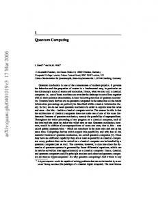
State transitions in a q-dimensional quantum system are performed by unitary quantum transformations, associated to square matrices of order 2q . The matrix notation of Hadamard and Pauly X transformations are defined by     1 1 1 0 1 √ H= and X= , 1 −1 1 0 2 respectively. By applying a Hadamard transformation to a quantum state |ψi, denoted by H|ψi, a new global state is obtained as follows:       1 1 α 1 1 α+β √ =√ × . β 1 −1 α−β 2 2 Quantum transformations simultaneously applied to different qubits imply on the tensor product of the corresponding matrices, as described in (3).     1 1 1 1 1 1 ⊗√ H ⊗2 = √ 1 −1 2 2  1 −1  1 1 1 1  1 1 −1 1 −1  . (3) = 1 −1 −1  2 1 1 −1 −1 1 In addition to the transformations obtained by the tensor product, controlled transformations can also modify one or more qubits. The CNOT transformation receives the tensor product of two qubits |ψi and |ϕi as input and applies the NOT (Pauly X ) transformation to one of them (target qubit), considering the current state of the other one (control), as illustrated by Fig. 1(a). The corresponding representation (quantum gates) in the quantum circuit model is presented in Fig. 1(b). Controlled transformations can be generalized (Toffoli ) in a similar way [1].

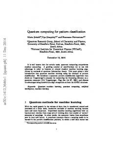
B. GPU Computing The parallel architecture of GPUs offers great computational power and high memory bandwidth, being suitable for accelerating many applications since a large number of processors (cores) is available. The CUDA programming model provides abstractions such as threads, grids, shared memory space, and synchronization barriers to help programmers to efficiently explore all resources available. It is based on the C/C++ language with some extensions for accessing GPU’s internal components. Programs are divided in a host-code and a device-code. The former, running on a CPU, consists of non-intense and mostly sequential computational loads. It is used to prepare the structures to run on the GPU and eventually for a basic pre-processing phase. The device-code runs on the GPU itself, representing the parallel portion of the related problem. Although the CUDA programming model is based on the C/C++ language, other languages and libraries are supported. In this work, the extension for Python language, named PyCuda [10], was chosen over a lower-level, better-performance language due to the following reasons: • Prototyping with the Python language is faster and easier due to its low coding restrictions; • The VPE-qGM environment is developed in Python and therefore an extension of its execution library to support GPUs execution is easily obtained; • The host-code is comprised of methods for the creation of the basic structures that later are copied to the GPU. Such creation is based on string formatting and manipulation of multidimensional structures, which can be easily prototyped with Python. On the other hand, the device-code perform a more restrictive and intensive computation, which is implemented in the C language as a regular CUDA kernel. By using the features of PyCuda, the technical challenges of the development process are reduced and greater attention is given to the algorithmic problem. A basic PyCuda workflow is shown in the Fig. 2. Binary executables are obtained from a C-like CUDA source code (CUDA kernel) generated from PyCuda as a string, allowing runtime code generation. The kernel is also compiled during runtime and stored in a semi-permanent cache for future reuse, if the source code is not modified.

(a) Matrix notation

(b) Quantum circuit Figure 1.

CNOT transformation

Figure 2.

Basic PyCuda compilation workflow [10]

III. Related Work Nowadays, quantum simulators with different approaches are available. The most relevant are described in the next sections, representing the best solutions achieved so far for parallel simulation of quantum algorithms. A. Massive Parallel Quantum Computer Simulator The Massive Parallel Quantum Computer Simulator (MPQCS) described in [4] is a parallel simulation software for quantum simulation. The simulations can be performed over high-end parallel machines or clusters of off-the-shelf desktops. Algorithms can be described through a universal set of quantum transformations, e.g. {H, S, T, CN OT }. Through combinations of these transformations, it is possible to describe any quantum algorithm. When using any universal set of transformations, limitations in the development process arise, since more complex operations must be specified only in terms of those transformations. However, this simplicity allows the application of more aggressive optimizations in the simulator, as the patterns of the computations are more predictable. Since the MPQCS explored the distributed simulation to improve the simulation, the MPI (Message Passing Interface) is used to send the data through the network to all connected nodes. The downside of this approach is the overload of the interconnection system due to the large amount of data transfered during the simulation. As the interconnection is used to send data related to the state vector of the quantum system to the corresponding processing nodes, and such state vector grows exponentially, a high capacity interconnection is preferred. The MPQCS simulator was executed in supercomputers such as IBM BlueGene/L, Cray X1E, IBM Regatta p690+, and others. The main results were a simulation of algorithms up to 36 qubits, requiring approximately 1 TB of RAM memory and 4096 processors. In 2010, as published in [11], the simulation of the Shor’s algorithm was performed on the JUGENE supercomputer, factoring the number 15707 into 113 × 139. Such task required 262.144 processors. The execution time and memory consumption were not published. B. General-Purpose Parallel Simulator for Quantum Computing The General-Purpose Parallel Simulator for Quantum Computing (GPPSQC), according with [5], is a parallel quantum simulator for shared-memory environments. The parallelization technique relies on the partition of the matrix of the quantum transformation into smaller sub-matrices. Those sub-matrices are then multiplied, in parallel, by sub-vectors corresponding to partitions of the state vector of the quantum system. The simulator also considers an error model that allows the insertion of minor deviations into the definition of the quantum transformations in order to simulate the effects of the decoherence in the algorithms.

By using the parallel computer Sun Enterprise (E4500), with 8 UltraSPARC-II (400MHz) processors, 1 MB cache, 10 GB of RAM memory and operational system Solaris 2.8 (64 bits), systems up to 29 qubits were supported. The results containing the simulation time (expressed in seconds) required for Hadamard gates, from 20 to 29 qubits are described in Fig. 3. As it can be seen, speedups of 5.12× were obtained for a 29-qubit Hadamard transformation using 8 processing cores.

Figure 3.

Simulation time, on seconds, for Hadamard gates [5].

C. Quantum Computer Simulation Using the CUDA Programming Language The quantum simulator described in [12] uses the CUDA framework to explore the parallel nature of quantum algorithms. In this approach, the computations related to the evolution of the quantum system are performed by thousands of threads inside a GPU. This approach considers a defined set of one-qubit and two-qubit transformations, being a more general solution in terms of transformations supported when comparing to the proposals of [4] and [5]. The use of a more expressive set of quantum transformations expands the possibilities for describing the computations of a quantum algorithm. As main limitations of the quantum simulation with GPUs, memory capacity is the more restrictive one, limiting the simulation presented by [12] to systems with a maximum of 26 qubits. As an important motivation towards this approach, the simulation time can achieve speedups of 95× against a very optimized CPU simulation. IV. VPE-qGM Environment The VPE-qGM environment is being developed in order to support the modeling and the simulation of algorithms from QC under the abstractions of the qGM model. An architectural overview of the entire environment that embraces this work is shown in Fig. 4, where three main components can be highlighted: • qPE (Quantum Process Editor): IDE where algorithms are graphically developed; • qME (Quantum Memory Editor): interface for the definition of the state vector. A memory grid stores each basic state and corresponding amplitude; • qS (Quantum Simulator): From the structures defined in the qPE and qME, the qS interface performs the simulation of a quantum algorithm, supporting

sequential and distributed simulation obtained by integration with the VirD-GM (Virtual Distributed Geometric Machine), as described in [6] and [13].

simulation. The later consists of modules resulting in a transparent manager responsible for the communication, synchronization and updating of results during the simulation. The distributed execution in the VirD-GM is controlled by three main modules. The VirD-Loader is responsible for the interpretation of descriptor files containing the algorithm to be simulated and its initial state vector. Scheduling and flux controlling are handled by the VirDLauncher module. Finally, the VirD-Exec module controls the communication and data movement between the execution clients, named VirD-Clients. The simulation aided by the VirD-GM consists in splitting equally the computation across the VirD-Clients. For example, in a quantum system with 10 qubits and 4 VirDClients, each VirD-Client generates 28 amplitudes of the new state vector according with the algorithm in Fig. 5. The M atrices variable contains a list of matrices with

Figure 4. Architectural overview of the qGM Quantum Simulation Environment

The qGM-Analyzer library, which is integrated with the qS simulator, performs the computation corresponding to the components that describe each step of a quantum algorithm. The support for the GPU acceleration is established in this library. The parallel simulation with GPUs resulting from this work represents a new simulation possibility for the VPE-qGM environment. The quantum circuit editor named QCEdit, proposed in [14], is also an important feature of the VPE-qGM environment. It allows the development of quantum computing simulations even without knowledge of the qGM model. Its related mobile extension, named as Mobile Quantum Circuit Editor and denoted by m-qCEdit, allows that quantum circuits modeled on mobile devices may be remotely simulated in a distributed way by the VPEqGM. The m-QCEdit consolidation brings together the facilities provided by the use of mobile devices to the intuitiveness of quantum circuits added to the possibility of parallel and/or distributed simulation on the VPE-qGM and VirD-GM, respectively. A. Distributed Simulation with the VPE-qGM The VPE-qGM environment supports the distributed simulation of quantum algorithms due to its integration with the VirD-GM environment. The former is a graphical environment focused on the interaction with the programmer during the development of the algorithm and its

if matrixIndex = numM atrices − 1 then for l = 0 to size(M atrices[matrixIndex]) do res ← 0; line ← M atrices[matrixIndex][l][1]; lineP os ← M atrices[matrixIndex][l][0]; for column = 0 to size(line) do pos ← baseP os + line[column][1]; res ← res + (partialV alue × line[column][0] × memory[1][pos]); end for writeP os ← memP os + (lineP os × sizesList[matrixIndex]); res ← res + memory[0][writeP os]; memory[0][writeP os] ← res; end for else for l = 0 to size(M atrices[matrixIndex]) do line ← M atrices[matrixIndex][l][1]; lineP os ← M atrices[matrixIndex][l][0]; for column = 0 to size(line) do ← baseP os + (line[column][1] × next baseP os sizesList[matrixIndex]); next partialV alue ← partialV alue × line[column][0]; ApplyV alues(M atrices, numM atrices, sizesList, memory, next partialV alue, matrixIndex + 1, next baseP os, memP os + (lineP os × sizesList[matrixIndex])); end for end for end if

Figure 5.

Execution algorithm for the VirD-Clients

dimensions in between 1 × 32 and 128 × 128. These matrices are generated from XML files that are automatically sent from the VPE-qGM environment when a distributed simulation is initiated. The dimensions of those matrices are dynamically defined considering the number of VirDClients available for the simulation. As an example, in a system with 10 qubits and 4 VirD-Clients, four XML files are generated and sent to four different VirD-Clients, creating matrices with dimensions {8 × 32, 32 × 32}. The lines of each matrix associated with the VirD-Client are defined as V irD − Client V irD − Client V irD − Client V irD − Client

1 = {[0, 7][0, 31]} 2 = {[8, 15][0, 31]} 3 = {[16, 23][0, 31]} 4 = {[24, 31][0, 31]}.

(4)

Each matrix is structured as follows:  Index      0  1 M=   ..    .  31

 M atrix Def inition     (α0 , 0) (α1 , 1) . . . (α30 , 30) (α31 , 31)   (β0 , 0) (β1 , 1) . . . (β30 , 30) (β31 , 31)   .. .. .. .. ..    . . . . .  (γ0 , 0) (γ1 , 1) . . . (γ30 , 30) (γ31 , 31)

•

(5)

The Index value identifies the lines of a matrix, since some of its lines may be hidden due to specifications regarding QP s and QP P s. The first element in each tuple of the M atrix Def inition indicates the actual complex value associated with the definition of the quantum transformation which is being applied. The second element is an index for the position occupied by the corresponding value, which is used to identify the amplitude of the state vector that must be multiplied by the final complex value generated in the base case of the recursive algorithm in Fig. 5. V. QC Simulation on the VPE-qGM using GPUs Considering all the features already added to the VPEqGM environment, an important contribution resulting from this work is the support for running simulations in GPUs. This section proposes a solution to the shortcomings discussed in the previous Section. A. Block and Grid Configuration The computation required by each CUDA thread comprehends the individual computation of 4 amplitudes of a new state vector. For a generic q-dimensional quantum transformation, the number of CUDA threads that are q necessary is defined by nT hreads = 24 . Each block has the static configuration of blockDim = (256, 1, 1), Consequently, the grid is defined as gridDim = ( nT hreads , 1, 1). 256 B. Constant-Size Source Matrices and Auxiliary Data Following the specifications in [9], a QP may be defined by building small-size matrices that are combined by an iterative function in order to dynamically generate the elements corresponding to the matrix, which is obtained whenever the Kronecker Product between the initial matrices was performed. For the execution of a QP, the system makes use of the following parameters and all of them are stored in a NumPy ’array’ object: • List of Matrices (matrices): matrices generated by the host-code; • List of Positions (positions): position of an element in the corresponding matrix is necessary to identify the amplitude of the state vector that will be accessed during simulation; • Width of Matrices (width): number of columns and also considering the occurrence of zero-values and the original dimension of the matrices; • Column Size of Matrices (columns): number of nonzero elements in each column; • Multiplicatives (mult): related to auxiliary values indexing the amplitude of the state vector;

Previous Values (previousElements): number of elements stored in the previous matrices.

C. Allocation of Data into the GPU When allocating structures into the GPU, data must be stored in the most suitable memory space (global memory, shared memory, constant memory and texture memory) to achieve good performance. As the QP parameters remain unchanged during an execution, they are allocated into the GPU’s constant memory. Such data movement is performed by PyCuda as described in the following steps: 1) In the CUDA kernel, constant data is identified according with the following syntax: device constant dT ype variable[arraySize]; 2) The device-memory address of variable is obtained in the host-code by applying the PyCuda call: address = kernel.get global(′ variable′ )[0]; 3) Data copy is also performed in the host-code in order to transfer the data stored in the host-memory to the device-memory address corresponding to variable. Such process is performed by the PyCuda call: pycuda.driver.memcpy htod(address, dataSource). Notice that dataSource is a NumPy [15] object stored in the host memory. This procedure is done for all variables cited in the Subsection V-B. Furthermore, the host-code contains two NumPy ’array’ objects that store the current state vector (readMemory) and the resulting state vector (writeMemory) after the application of the quantum transformations. Additionally, the parameter writeMemory has all its positions zeroed before each step of the simulation. Next, the data related to readMemory and writeMemory are copied to the global memory space of the GPU. The following methods consolidate such process: 1) readM emory = numpy.array(numpy.zeros(2q ), dtype = numpy.complex64, order =′ C ′ ) is related to a NumPy array creation, with all its values equal to zero and resides in the host side. The desired current state is then manually configured. 2) readM emory gpu = gpuarray.to gpu(readM emory) represents the copy of the current (input) state vector from the host-memory to the device-memory through a PyCuda call. 3) writeM emory gpu = gpuarray.zeros(2q , dtype = numpy.complex64, order =′ C ′ ) is the new (output) state vector of the system, only created in the device side and initialized with all its values equal to zero by a PyCuda call. D. CUDA Kernel The CUDA kernel is an adaptation of the recursive algorithm presented in Fig. 5 to an iterative procedure, as GPUs’ kernels can not contain recursive calls. As this kernel is inspired by the Kronecker Product, it operates over an arbitrary number of source matrices. Each CUDA

thread has its own internal stack and iteration control to define the access limits inside each matrix. The computation of each thread can be depicted in seven steps, described as follows. Step 1 performs the initialization of variables in the constant memory, which are common to all CUDA threads launched by a kernel. T OT AL ELEM EN T S , LAST M AT RIX ELEM EN T S and ST ACK SIZE are defined in runtime by the PyCuda interpreter. For text formatting purposes, this Subsection considers the symbol ⋄ as a representation of the declaration device constant . ⋄ cuF loatComplex matricesC[T OT AL ELEM EN T S]; ⋄ int positionsC[T OT AL ELEM EN T S]; ⋄ cuF loatComplex lastM atrixC[LAST M AT RIX ELEM EN T S]; ⋄ int lastP ositionsC[LAST M AT RIX ELEM EN T S]; ⋄ int widthC[ST ACK SIZE + 1]; ⋄ int multC[ST ACK SIZE + 1]; ⋄ int columnsC[ST ACK SIZE + 1]; ⋄ int previousElementsC[ST ACK SIZE + 1];

Step 2 consists in shared memory allocation and initialization performed by all CUDA threads within a block. SHARED SIZE is defined in run-time by the PyCuda interpreter, which in general will assume the value blockDim.x × 4. shared

cuF loatComplex newAmplitudes[SHARED SIZE];

f or (int i = 0; i < 4; i + +){ ind = threadIdx.x × 4 + i; newAmplitudes[ind] = make cuF loatComplex(0, 0); } syncthreads();

Step 3 defines the access limits of a matrix, determining which elements each CUDA thread will access depending on its id and resident block. The begin, count and end arrays are local to each thread and help the controlling and indexation of the elements of each matrix in matricesC and positionsC. The (thId&(widthC[c] − 1)) operation is analogous to the module operation thId%widthC[c] but performed as a bitwise ′ and′ that is more efficient in the GPU int thId = blockDim.x × blockIdx.x + threadIdx.x; f or(int c = ST ACK SIZE − 1; c > −1; c − −){ begin[c] = (thId&(widthC[c] − 1)) × columnsC[c]; count[c] = begin[c]; end[c] = begin[c] + columnsC[c]; thId = f loorf ((thId/widthC[c])); }

Step 4 is responsible for forwarding in matrices, which is analogous to a recursive step, providing the partial multiplications among the current elements according to the indexes in count. while (ind < ST ACK SIZE){ position = positionsC[previousElementsC[ind]]; mod = (position + count[ind])&(widthC[ind] − 1); readStack[top + 1] = readStack[top] + (mod × multC[ind]); of f set = previousElementsC[ind]; element = matricesC[of f set + count[ind]]; valueStack[top + 1] = cuCmulf (valueStack[top], element); top + +; ind + +; }

Step 5 performs the shared memory writing, related to a partial update of the amplitude in the state vector. c = 0; f or(int j = 0; j < 4; j + +){ res = make cuF loatComplex(0, 0); f or(int k = 0; k < columnsC[ST ACK SIZE]; k + +){ mod = (lastP ositionsC[c]&(widthC[ind] − 1)) readP os = readStack[top] + mod; mult = cuCmulf (lastM atrixC[c], readM emory[readP os]); res = cuCaddf (res, mult); c + +; } writeP os = threadIdx.x × 4 + j; partAmp1 = newAmplitudes[writeP os]; partAmp2 = cuCmulf (res, valueStack[top]); newAmplitudes[writeP os] = cuCaddf (partAmp1, partAmp2); }

Step 6 changes the index in previous matrices, generating the next values associated to the resulting matrix. This process continue until all the indexes reach the last element of the corresponding line in all matrices. top − −; ind − −; count[ind] + +; while(count[ind] == end[ind]{ count[ind] = begin[ind]; ind − −; count[ind] + +; top − −; }

Step 7 copies the data from shared memory to global memory after all CUDA threads have finished their calculations. thId = blockDim.x × blockIdx.x + threadIdx.x; f or (int i = 0; i < 4; i + +){ writeP os = thId × 4 + i; readP os = threadIdx.x × 4 + i; writeM emory[writeP os] = newAmplitudes[readP os];

VI. Results The analysis of the parallel simulation using GPUs is based on the simulation of Hadamard transformations, always considering the global state of the quantum system. In order to compare the performance of this new proposal, the results of the distributed simulation obtained by the VirD-GM are used as reference as they represent the best performance achieved in this project until now. The distributed simulation was performed using two nodes with the following configuration: Intel Quad2Core Q8200 2, 33GHz processor, 4 GB RAM, Fast Ethernet network and Ubuntu 12.04 64 bits operational system. An additional machine was required to run the VirD-GM server. The methodology for the distributed simulation considers the execution of 15 simulations of each instance of the Hadamard transformations, considering each one of the configurations of processing cores within the cluster.

For the simulation with GPUs, the tests were performed on a desktop with an Intel Core i7-3770 processor, 8 GB RAM, and a NVIDIA GT640 GPU. The software components are: PyCuda 2012.1 (stable version), NVIDIA CUDA 5, NVIDIA Visual Profiler 5.0 and Ubuntu 12.04 64 bits. There were simulated Hadamard transformations up to 20 qubits. The simulation time was obtained with the NVIDIA Visual Profiler after 30 executions of each application. Table I contains the simulation time, in seconds, for Hadamard transformations ranging from 14 to to 20 qubits, considering the distributed simulation by the VirDGM and the parallel simulation using GPUs proposed in this work. The results in Table I represent a significant Table I Simulation time, in seconds, for the distributed simulation using the VirD-GM and the parallel simulation using GPUs

H ⊗14 H ⊗15 H ⊗16 H ⊗17 H ⊗18 H ⊗19 H ⊗20

1 core 3.45·101 1.34·102 5.42·102 2.19·103 1.01·104 -

2 cores 1.81·101 7.05·101 2.83·102 1.13·103 5.40·103 -

4 cores 1.19·101 4.23·101 1.71·102 6.92·102 3.13·103 -

8 cores 0.67·101 2.26·101 8.69·101 3.51·102 1.59·103 -

GPU 0.08 0.29 1.15 4.59 1.87·101 7.57·101 3.14·102

performance improvement when using a GPU. The standard deviation for the simulation time collected related to the distributed simulation has reached a maximum value of 1.9% for the H ⊗18 executed with 1 and 8 cores. A complete 8-core simulation of the configurations with 19 and 20 qubits would require approximately 1 and 5 hours, respectively. Due to such simulation time, those case studies were not simulated in the VirD-GM. The speedups presented in Fig. 6 have reached a maximum of ≈ 540× when comparing with the 1-core execution in the VirD-GM. The GPU-based simulation has outperformed the best distributed simulation in the VirDGM by a factor of ≈ 85× for the Hadamard of 18 qubits running on 8 processing cores. This improvement is justified by the number of CUDA cores (384) available in the GPU explored in this work. As the distributed simulation performed by VirD-GM does not consider further optimizations regarding memory access and off-the-shelf desktops and network interfaces were used, performance obtained by the GPU execution was much better. More significantly, applications with more than 18 qubits require at least 8 processing cores for distributed simulation with the VirD-GM environment. For the parallel simulation with GPUs, a 20-qubit Hadamard can be simulated with one mid-end device, such as a NVIDIA GT640. Regarding the GPU’s execution, the NVIDIA Visual Profiler has identified a local memory overhead associated with the memory traffic between the L1 and L2 caches, caused by global memory access corresponding to the reads

Figure 6. Speedups for the GPU simulation relative to the number of cores considered in the distributed simulation by the VirD-GM

in the readM emory variable, as described in the Step 5 presented in the Subsection V-D. From the results mentioned above, the performance improvement obtained in comparison with the distributed simulation in the VirD-GM is evident. However, the GPU simulation proposed in this has two constraints. The first is related to the memory space required for the simulation. As the state space of the quantum system grows exponentially, and it is entirely stored in the global memory of the GPU, the simulation would be limited to systems up to 25 qubits, if running on a GPU with 1 GB of RAM memory. The second limitation is due to the exponential increase in the simulation time. As an example, our current solution would require ≈ 1.26 · 106 seconds to perform a simulation of a Hadamard transformation applied to 25 qubits. In order to overcome such limitations, our research is currently focusing on solutions for both of those problems. VII. Conclusions The simulation of quantum algorithms using classical computers presents high temporal and spatial complexities. In order to establish the foundations for a new solution to deal with such limitations, this work introduces an extension of the qGM-Analyzer library that allows the use of GPUs to accelerate the simulation algorithm of the VPE-qGM. The contribution of this proposal to the environment already established around the VPE-qGM intends to lead to simulations of quantum algorithms on clusters of GPUs. Although the support for simulation of quantum transformations using GPUs described in this work is in its initial stages, it has already significantly improved the simulation capabilities of the VPE-qGM. Speedups of ≈ 85× related to a 8-core distributed simulation, and of ≈ 540× related to the 1-core simulation were obtained when comparing this novel solution to the distributed simulation provided by the VirD-GM environment. Simulations of Hadamard transformations up to 20

qubits were performed. Without the contributions of this work, such simulation could not be done in the VPEqGM due to the elevated execution time. The Hadamard transformation was chosen as a case study in this work because of its high computational cost and represents the worst case scenario for the simulation in this environment. In this work only simulations with Hadamard transformations were performed since the development is in its early stages. However, the guidelines for the next step of the research are already established and published in [16], where the sequential simulation was performed considering several quantum algorithms. As a result, algorithms described by controlled transformations up to 24 qubits were simulated in ≈ 1500 seconds. Those results motivate our group in the pursuit of even better results on the GPU. When comparing the results of our proposal with related works, it is expected that other simulators will outperform our current solutions due to two main reasons: • Current solutions consider a restricted set of quantum operations, which simplify the optimizations for the simulation but impose restrictions during the development of a quantum algorithm. Our solution consists in a generic approach in order to support any unitary quantum transformation; • Data in the GPU’s global memory is often accessed. By moving sections of such data to the GPU’s shared memory and partitioning the computation of the CUDA threads in sub-steps to control memory access, performance can be improved. Future work will consider several algorithmic optimizations that will be applied to reduce the number of computations, where the following ones can be highlighted: • As the matrices that define quantum transformations are orthogonal, only the superior (or inferior) triangle can be considered in the computations. The most significant impact expected is the decrease of memory accesses and required storage. Reductions in the number of computations is also possible; • A more sophisticated kernel that predicts multiplications by zero-value amplitudes of the state vector may avoid unnecessary operations. A major reduction in the number of computations is expected; • Establish the support for simulations using clusters of GPUs through the extension of the VirD-GM environment. Acknowledgment This work is supported by the Brazilian funding agencies CAPES, FAPERGS (Ed. PqG 06/2010, under the process number 11/1520-1), and by the CNPq/PRONEX/FAPERGS Green Grid project. References [1] M. A. Nielsen and I. L. Chuang, Quantum Computation and Quantum Information. Cambridge University Press, 2000.

[2] L. Grover, “A fast quantum mechanical algorithm for database search,” Proceedings of the Twenty-Eighth Annual ACM Symposium on Theory of Computing, pp. 212–219, 1996. [3] P. Shor, “Polynomial-time algoritms for prime factorization and discrete logarithms on a quantum computer,” SIAM Journal on Computing, 1997. [4] K. D. Raedt, K. Michielsen, H. D. Raedt, B. Trieu, G. Arnold, M. Richter, T. Lippert, H. Watanabe, and N. Ito, “Massive parallel quantum computer simulator,” http://arxiv.org/abs/quant-ph/0608239, 2006. [5] J. Niwa, K. Matsumoto, and H. Imai, “General-purpose parallel simulator for quantum computing,” Lecture Notes in Computer Science, vol. 2509, pp. 230–249, 2008. [6] A. Maron, A. Pinheiro, R. Reiser, and M. Pilla, “Distributed quantum simulation on the VPE-qGM,” in WSCAD-SSC 2010. IEEE Computer Society - Conference Publishing Services, 2010, pp. 128–135. [7] NVIDIA, NVIDIA CUDA C Programming Guide. NVIDIA Corp., 2012, version 4.2. [8] R. Reiser and R. Amaral, “The quantum states space in the qGM model,” in Proc. of the III Workshop-School on Quantum Computation and Quantum Information. Petr´ opolis/RJ: LNCC Publisher, 2010, pp. 92–101. [9] A. Maron, R. Reiser, M. Pilla, and A. Yamin, “Quantum processes: A new approach for interpretation of quantum gates in the VPE-qGM environment,” in Proceedings of WECIQ 2012, 2012, pp. 80–89. [10] A. Kloeckner, “Pycuda online documentation,” 2012, http://documen.tician.de/pycuda/. [11] M. Henkel, “Quantum computer simulation: New world record on jugene,” 2010, available at http://www.hpcwire.com/hpcwire/2010-06-28/ quantum computer simulation new world record on jugene.html (feb. 2013). [12] E. Gutierrez, S. Romero, M. Trenas, and E. Zapata, “Quantum computer simulation using the cuda programming model,” Computer Physics Communications, pp. 283–300, 2010. [13] V. Fonseca, R. Reiser, A. Yamin, and P. Pilla, “VirD-GM: Towards a grid computing environment,” in Proceedings of CCGRID 2007, 2007, pp. 1–6. ´ [14] A. Maron, A. Avila, R. Reiser, and M. Pilla, “Specifying a basic architecture for converting quantum circuits to the qGM model,” in Proceedings of the Worshop on Free Software 2011, 2011, pp. 1–6. [15] N. community, “NumPy user guide - release 1.6.0,” 2011, http://docs.scipy.org/doc/numpy/numpy-user.pdf. [16] A. Maron, A., R. Reiser, M. Pilla, and A. Yamin, “Quantum processes: A new interpretation for quantum transformations in the VPE-qGM environment,” in CLEI 2012. IEEE Computer Society - Conference Publishing Services, 2012, pp. 1–10.