network and parallel I/O support. To study the performance of this rendering pipeline and to demonstrate high-performance remote visualization, tests.
High Performance Visualization of Time-Varying Volume Data over a Wide-Area Network Kwan-Liu Ma
David M. Camp
University of California-Davis�
Abstract This paper presents an end-to-end, low-cost solution for visualizing time-varying volume data rendered on a parallel computer located at a remote site. Pipelining and careful grouping of processors are used to hide I/O time and to maximize processors utilization. Compression is used to significantly cut down the cost of transferring output images from the parallel computer to a display device through a wide-area network. This complete rendering pipeline makes possible highly efficient rendering and remote viewing of high resolution time-varying data sets in the absence of high-speed network and parallel I/O support. To study the performance of this rendering pipeline and to demonstrate high-performance remote visualization, tests were conducted on a PC cluster in Japan as well as an SGI Origin 2000 operated at the NASA Ames Research Center with the display located at UC Davis. Keywords: High Performance Computing, Image Compression, Parallel Volume Rendering, Pipelining, Remote Visualization, Scientific Visualization, Time-Varying Data, Wide-Area Network
1 Introduction The ability to study time-varying phenomena helps scientists understand complex problems. Time-varying volume data sets, which may be obtained from numerical simulations or remote sensing instruments, provide scientists insights into the detailed dynamics of the phenomenon under study. When appropriately rendered, they form an animation sequence that can illustrate how the underlying structures evolve over time. A typical time-varying data set from a computational fluid dynamics simulation can contain hundreds to thousands of time steps and each time step can easily have more than millions of data points. It can take gigabytes to terabytes of storage space to store a single data set. Scientists run this type of large scale numerical simulations on parallel supercomputers operated at a government research laboratory or � Center for Image Processing and Integrated Computing (CIPIC), Department of Computer Science, University of California, One Shields Avenue, Davis, CA 95616-8562, e-mail: {ma,campd}@cs.ucdavis.edu
0-7803-9802-5/2000/$10.00 c 2000 IEEE.
a national supercomputer center. Moving a complete timevarying data set from the supercomputer center to the scientist’s own computing laboratory for data analysis and visualization, if not impossible, can be very troublesome. There are better approaches to this problem. One is based on a runtime visualization scenario, and the other is a postprocessing visualization scenario. Visualizing time-varying data probably can be done most efficiently while the data are being generated, so that users receive immediate feedback on the subject under study, and so the visualization results can be stored rather than the much larger raw data. However, runtime tracking is not always possible and desirable for certain applications. For example, one may want to explore the data set from different perspectives; or, the amount of computation power required for real-time rendering or a special visualization technique may not be readily available. Most importantly, competing with the numerical simulation to perform visualization calculations for computing time and memory space on the same parallel supercomputer is generally not acceptable by many scientists. As a result, postprocessing of pre-calculated data remains an important requirement, and the scenario is that the scientist leaves the data on the supercomputer center’s mass storage device, retrieves them to perform visualization calculations on a parallel computer at the supercomputer center, and displays the resulting images/animations on his/her desktop computer. While this might have been a common practice for many supercomputers’ users, the ability to visualize time-varying data over a wide-area network in an interactive manner is still absent. Two obstacles are: 1) visualizing time-varying data requires reading large files continuously or periodically throughout the course of the visualization process, and 2) the delay due to transferring the resulting (preferably high resolution) images over a wide-area network makes it impossible to achieve interactive viewing even though the parallel computer used can render at multiple frames per second. In this paper, we present a low-cost solution combining pipelining, efficient processor management and compression to achieve near-interactive remote visualization of timevarying data on a parallel computer. This new capability we offer to computational scientists can lead to more productive study of large-scale time-varying problems in the absence of high-speed network and parallel I/O support.
2 Previous Work 2.1 Time-varying data visualization Runtime visualization of time-dependent simulations has been demonstrated by several researchers. Rowlan [22] and Ma [14] independently demonstrated runtime tracking of three-dimensional numerical simulations using direct volume rendering on a massively parallel computer. VISUAL3 [7] and SCIRun [21] are among a few software systems that can support runtime tracking. These systems can be operated in a distributed computing environment. Many techniques have been developed for visualizing time-varying data as a postprocess. Lane [13] developed a particle tracer for three-dimensional time-dependent flow data. Max and Becker [18] applied textures to visualize both steady and unsteady flow fields. Silver and Wang [26] present a volume based feature tracking algorithm to help visualize and analyze large time-varying data sets. Jaswal [9] demonstrates distributed real-time visualization of timevarying data using a CAVE. Encoding methods for time-varying data have also been investigated to facilitate interactive visualization. Shen and Johnson [25] develop a ray-casting volume rendering strategy by exploiting the data coherency between consecutive time steps, and they are able to reduce not only the rendering time but also the storage space by 90% for their two test data sets. More recently, Shen, Chiang and Ma [24] proposed a new data structure called time-space partitioning (TSP) tree to effectively capture both the spatial and temporal coherence from time-varying fields for volume rendering calculations. Sutton and Hansen [28] used a temporal Branch-onNeed tree for efficient isosurface extraction in time-varying fields.
2.2 High performance visualization systems High performance visualization of large data sets can be achieved by leveraging advanced data processing and visualization techniques on state-of-the-art hardware equipment including massively parallel computers, parallel I/O and high speed network support, multiprocessor graphics workstations, and dedicated frame buffer. To attain the highest possible overall system efficiency, integration is the key. McPherson and Maltrud [19] demonstrated interactive ocean model visualization by utilizing high speed graphics hardware, and intend to implement data streaming to achieve out-of-core processing. MPIRE (http://mpire.sdsc.edu/) is a volume rendering server, which allows the user to select a rendering method (splatting or ray casting), rendering parameters, and a parallel rendering engine (Cray T3D, Cray T3E, or SGI multiprocessor Workstation) through a javabased graphical user interface (or an AVS module). Heermann [8] realized a production visualization system with improved hardware and software to speed up every stage in the visualization pipeline. Parker, et al. [20] developed an inter-
active ray-tracing renderer on a distributed shared memory multiprocessor machine for volume visualization. A recent effort is the the development of visualization corridors [27] focusing an integrated solution for “distance visualization.” Turning to the I/O issue, work has been done mainly addressing the I/O characteristics of graphics and visualization applications on parallel computers [4, 23, 3]. The parallel I/O capabilities of MPI-2 [6] offer a standard way to implement high performance I/O which allows noncontiguous access patterns and collective I/O. Kotz maintains an online archive (http://www.cs.dartmouth.edu/pario/) providing abundant information about the research on and the use of Parallel I/O. The work described here, in contrast, focuses on a generic software solution. We assume no dedicated frame buffer, high-speed network, parallel I/O support, nor high-end graphics hardware. We investigate how resource utilization, compression and parallelism can optimize the overall remote visualization process.
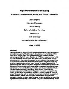
3 Parallel Pipelined Rendering The basic structure of a complete parallel volume rendering pipeline consists of four stages as shown in Figure 1. The data-input stage reads data from disk and distributes them to the processor nodes. Each processor receives a subset of the volume data. In the local rendering stage, each processor node renders the assigned subvolume into a 2D partial image independent of other processors. In the following global image compositing stage, which generally requires interprocessor communication, the set of 2D partial images are composited according to the view position to arrive at the final 2D projected image. Finally, in the image-output stage the rendered image is delivered to a display device. When the degree of parallelism is small to modest, e.g., under 16 nodes, the major portion of the computational cost is attributed to subvolume rendering. However, when the degree of parallelism is high or when the data set itself is large (say 5123 or 10243 voxels per time step), 3D data distribution becomes a significant performance factor. Parallel rendering of time-varying data involves rendering multiple data volumes in a single task. There are three potential performance metrics: start-up latency, the time until the rendered image of the first volume appears; overall execution time, the time until the rendered image of the last volume appears; and inter-frame delay, the average time between the appearance of consecutive rendered images. In conventional volume rendering applications, since only one data set is involved, start-up latency and overall execution time are the same, and inter-frame delay is irrelevant. When interactive viewing is desired, start-up latency and inter-frame delay play crucial role in determining the effectiveness of the system. When visualization calculations are done in a batch mode, overall execution time should be the major concern.
Disk/Simulation
Data input Local rendering Global image compositing Image output Display/Storage Device Figure 1: A complete parallel volume rendering pipeline. To achieve interactive visualization of time-varying data, both the data-input stage and the image-output stage must be able to keep up with the rendering rates. Different design tradeoffs should be made for different performance criterion. Given a generic parallel volume renderer and a Pprocessor machine, there are three possible approaches to manage the processors for rendering time-varying data sets. The first approach simply runs the parallel volume renderer on the sequence of data sets one after another. At any point in time, the entire P-processor machine is dedicated to rendering a particular volume. That is, here we assume the pipeline effect is ignored. Therefore, only the parallelism associated with rendering a single data volume, i.e., intra-volume parallelism, has been exploited. The second approach takes the exact opposite approach by rendering P data volumes simultaneously, each on one processor. This approach thus only exploits inter-volume parallelism, and is limited by each processor’s main memory space. To attain the optimal rendering performance we should carefully balance two performance factors, resource utilization efficiency and parallelization overhead, which suggests exploiting both intra-volume and inter-volume parallelism. The third approach is thus a hybrid, in which P processor nodes are partitioned into L groups (1 < L < P), each of which renders one volume (i.e. one time step) at a time. The optimal choice of L generally depends on the type and scale of parallel machine as well as the size of data set. The optimal partitioning strategy for minimizing the overall rendering time can be characterized with a performance model and
revealed with an experimental study [15]. Our test results demonstrate that the third approach indeed performs the best among the three for batch-mode rendering. To achieve remote, interactive visualization over a widearea network, it becomes also important to minimize interframe delay. We investigate how processors partitioning can be optimized for better interactivity, and study the interplay between the renderer and the display strategy along with the data compression/transfer mechanism that we have developed.
4 Efficient Image Transfer The mix of pipelined rendering with processors grouping makes possible overlapping data input, rendering and image output, and therefore leads to optimal overall rendering performance in the absence of parallel I/O support. We assume that the volume data set is local to the parallel supercomputing facility, and is transmitted to the parallel renderer through fast LANs. The cost of the last stage of the pipeline - image output - cannot be ignored since the resulting images must be assembled and transported to the desired display device(s) with minimal delay, possibly over a wide-area network. The performance of a pipeline is determined by its slowest stage. Except with very a high speed network or low-resolution images, compression is required to deliver the desired frame rates. For parallel rendering applications, we need image compression techniques which will compress with reasonable speed, exhibit good compression with short input strings, accept arbitrary orderings of input data, and decompress rapidly. The choice of compression technique will also be influenced by factors such as rendering performance, network bandwidth, and image accuracy/quality. To date, renderer implementations exploiting image compression have mostly adopted relatively simple lossless schemes which rely on frame-differencing and run-length encoding, in part because they satisfy many of the desired criteria. While these techniques can usually deliver several frames per second over local area networks (FDDI, Fast Ethernet, and even 10 Mb/s Ethernet), their compression ratios are highly dependent on image content, and are insufficient for use on slower widearea and long-haul networks. We are inclined to use lossy (visually lossless) compression methods capable of providing acceptable image quality for many applications, while retaining desirable properties such as efficient parallelizable compression, insensitivity to image organization, and, most importantly, rapid decompression.
4.1 A Framework for Image Transport Compression can be done collectively by the rendering nodes or by a dedicated node for efficient image transport. Parallel
Compute node
Image assembling
Data input
local network Disk
wide−area network Decompression and Display Remote User
Figure 2: A remote visualization system. Compression is used to accelerate image transport, and can be done by the image assembling node, or collectively by the compute nodes. compression would require decompression of multiple images at the receiving end which usually uses a less powerful machine. Figure 2 shows the architecture of the proposed system. “Parallel compression” can be realized in two different ways. One is to have each processor compress a portion of the image independent of other processors. The other is to have all the processors collectively compress an image which would require inter-processor communication. The later would give the best compression results in terms of both quality and efficiency, but it is a less portable solution. Parallelizing compression calculations is itself an interesting research problem [25], and the goal is to minimize communication cost as much as possible. In this study, we have only experimented with the former approach which is easy to implement and, as shown in the test results section, can achieve the needed efficiency for fast image transport. In general, our compression-based image output stage is based on a framework consisting of three parts: renderer interface, display interface, and display daemon. The renderer interface provides each rendering node with image compression (if not done by the renderer) and communication to and
from the display daemon. The display interface provides three basic functions: image decompression, image assembly, and communication to and from the display daemon. The communication path can instruct the system to change the compression method, start the renderer, or pass a message directly to the renderer. The display daemon’s main job is to pass images from the renderer to the display. It also allows the display to communicate with the renderer. In addition, the display daemon can accept any number of connections from renderer interface and display interface. We have studied several image compression methods and transport mechanisms. Interaction with the parallel renderer is provided by the display application. In our system, the user interface tasks are split between the controlling workstation and the parallel renderer. The display application drives the control panel display and passes events to the renderer though the display interface, which passes through the display daemon to all renderer interfaces in the form of "remote callbacks". The renderer responds with the appropriate action and may need to re-render the image.
4.2 Compression methods While image compression is a well developed field, continuing progress is being made due to the demand for higher compression performance from an increasing number of application areas. JPEG-2000 [17] is an emerging standard for still image compression, and MPEG [10] is for coding moving pictures. For our study, we have looked over several compression methods, both lossless and lossy ones. Low cost is one of our selection criteria. This eliminates JPEG-2000 (based on wavelet transform) because of its relatively high computational complexity even though it provides significantly lower distortion for the same bit-rate. JPEG-2000 also requires more memory than JPEG. Low decompression cost is particularly important since computing resources are generally low at the receiving end when considering our remote visualization setting. Rendering time-varying data produces an animation sequence. MPEG, which is good for compressing existing videos, is not suited for the interactive setting of ours in which each image is generated on the fly and to be displayed in real time. While using MPEG is not completely impossible, the overhead would be too high to make both the encoding and decoding efficient in software. Therefore, in our study, we mainly consider JPEG and two other compression methods, LZO and BZIP, with which we found worth experimenting. LZO does lossless data compression, and offers fast compression and very fast decompression. The decompression requires no extra memory. In addition there are slower compression levels achieving a quite competitive compression ratio while still decompressing at very high speed. In summary, LZO is well suitable for data de-/compression in real-time, which means it favors speed over compression ratio.
BZIP has very good lossless compression, better than gzip in compression and decompression time. BZIP compresses data using the Burrows-Wheeler block-sorting compression algorithm [2] and Huffman coding. Compression is generally considerably better than that achieved by more conventional LZ77/LZ78-based compressors, and approaches the performance of the PPM family of statistical compressors. JPEG (http://www.jpeg.org/) is designed for compressing full-color images of real-world scenes by exploiting known limitations of the human eye, notably the fact that small color changes are perceived less accurately than small changes in brightness. The most widely implemented JPEG subset is the “baseline” JPEG which provides lossy compression, though the user can control the degree of loss by adjusting certain parameters. Another important aspect of JPEG is that the decoder can also trade off decoding speed against image quality, by using fast but inaccurate approximations to the required calculations. Remarkable speedups for decompression can be achieved in this way. For our applications, JPEG thus provides the flexibility to cope with the required frame rates. The newer “lossless JPEG”, JPEG-LS, offers mathematically lossless compression. The decompressed output of the “baseline JPEG” we use can be visually indistinguishable from the original image. JPEG-LS gives better compression than original JPEG, but still nowhere near what you can get with a lossy method. Further discussion of compression methods can be found in many published reports and web sites, and is beyond the scope of this paper.
5 User Control To allow user control of the rendering and viewing, feedback from the user must be integrated into the pipelined rendering. The current framework is set up to allow the display client code to send a tagged message to the renderer engine. Rendering of current frames is not interrupted. Instead, the user inputs, which can be a new color map or a new viewing position, are buffered and only affect the rendering of following frames. Depending on the level of change in focus and context, certain delay is expected. Because true real-time viewing and manipulation is generally not possible anyway, we choose not to stop rendering calculations that have been started. More elaborated control mechanism will be needed if interactive manipulation is frequently needed. In this paper, no experimental results on user control is provided.
6 Experimental Results In this section, we present our findings, and demonstrate, with experimental results, remote, near-interactive visualization of time-varying volume data over a wide-area network. We conducted tests on two different parallel computers. One was an SGI Origin 2000 (O2K) located at the NASA Ames
Figure 3: Volume visualization of a numerically simulated turbulent jet. This data set consists of 150 time steps, and stores scalar vorticity on a regular mesh with 129�129�104 data points.
Research Center, about 120 miles from UC Davis. The other one was a PC cluster located at Japan. This PC cluster is operated at the Parallel and Distributed System Software Laboratory of the Real World Computing Partnership (RWCP) in Japan. It consists of 130 200 MHz Intel Pentium Pro microprocessors connected by a Myrinet giga-bit network. To test the remote rendering pipeline, the parallel computer was connected to an SGI O2 workstation at our Graphics Laboratory. Most of our timing results were obtained by averaging over a large number of tests. Three different fluid flow test data sets were used for our study. Because of the large number of tests we needed to perform and the limited computer time we had on the parallel computers, we used a small data set for the majority of the tests. This small data set consists of 150 time steps (129�129�104 data points each). Figure 3 displays an image of a particular time step in this data set. Another small data set of similar size has 100 time steps (1283 data points each) but with somewhat different image characteristics. Figure 4 displays a time step in this data set. Finally, a 265 time steps, 640�256�256 data set was used. Figure 5 displays a time step in this data set. These last two data sets were used to study selected aspects of the compression results and the parallel visualization pipeline. We use a parallel ray-casting volume renderer [16] for our study. This renderer is reasonably optimized and capable of generating high quality images. There are other volume rendering algorithms such as the shear warp algorithm [12] which can not only deliver superior rendering rates but is also highly parallelizable [11]. Since our task is to render time-varying data, the preprocessing calculations required by the shear warp algorithm must be done for every time step. This requirement makes the shear warp algorithm less attractive. Including the preprocessing time for each time step, a shear-warp image and a ray-cast image could take almost the same amount of time to generate. In addition, due to the use of 2-d filtering, the quality of a shear warp image, in some
Figure 6: The overall execution time versus the number of partitions for three different processor sizes on the RWCP PC cluster. The first 128 time steps of the turbulent jet data set was used. The output image size is 256�256 pixels. Figure 4: Volume visualization of turbulent vortex flow. The original data set was generated from a pseudo-spectral simulation of coherent turbulent vortex structures. The version of the data set that we obtained from Dr. Deborah Silver has 100 time steps and stores scalar vorticity magnitude on a regular mesh with 128�128�128 data points.
Figure 5: Volume visualization of data in the modeling of shock refraction and mixing. The initial condition of the simulation consists of an ambient medium with a bubble-shaped region containing a denser fluid. Over the course of the simulation, a shock wave in the ambient medium passes through the volumes, causing the two fluids to mix. This data set was computed by the Center for Computational Science and Engineering at NERSC. The version of the data set we obtained was resampled from an AMR mesh to a regular mesh of 640�256�256 data points. There are 265 time steps and three velocity components are stored at each data point. So the overall size of the data set is over 44 gigabytes.
case, could be less ideal. Our ray-casting renderer takes from about 10 to 20 seconds to generate an image of 256�256 pixels using a single processor. First, tests were performed on the RWCP cluster to reveal the relationship between the overall execution time and the number of processor partitions (L). Figure 6 displays the test results on a logarithmic scale along the x-axis. Our conjecture that the optimal performance can only be achieved by effectively exploiting both intra-volume and inter-volume parallelism is verified by the test results. An optimal partition does exist and it is four for all three processor sizes 16, 32, and 64. Figure 7 shows the behavior of the three performance metrics described earlier versus the degree of partitioning, and the tradeoff among them. The start-up latency monotonically increases with the number of partitions since fewer processors are dedicated to the rendering of a single data volume. Because of the dominance of the overall execution time, the inter-frame delay exhibits a somewhat similar curve as that associated with overall execution time. Next, Table 1 compares the compressed image sizes for the three compression methods we considered, and also a combination of them. When lossy compression is acceptable, JPEG is the choice because of the excellent compression it can achieve. Moreover, we found that using either LZO or BZIP to compress the output of JPEG can result in additional compression which may lead to the key reduction required for achieving the desired frame rates. We thus use this two-phase compression approach in our display system. The compression rates we have achieved are 96% and up. Although using, for example, LZO adds only additional 12% of compression, reducing the transferred image size by another couple of kilobytes effectively can increase frame
Overall Display Time for One Frame
35
Display Daemon
30
X Display 25
Inter-Frame Delay Time (sec)
Time (sec)
400 350 300 250 100 90 80 70 60 50 40 30 20 10 0
Start-up Latency Overall Time
20 15 10 5 0 128
256
512
1024
Image Size
1
2
4 8 16 Number of Partitions
32
Figure 8: Time to send one frame from NASA Ames to UCD via X or compression for displaying on a workstation.
Figure 7: The overall execution time, start-up latency, and average inter-frame delay versus the number of partitions, when P=32 for the RWCP cluster. Table 1: Compressed image sizes in bytes methodnimg size Raw LZO BZIP JPEG JPEG+LZO JPEG+BZIP
1282 49152 16666 12743 1509 1282 1642
2562 196608 63386 44867 3310 2667 3123
5122 786432 235045 152492 9184 6705 7131
10242 3145728 848090 482787 28764 18484 18252
rates. Figure 8 compares the time via two different display mechanisms: X-Window and our compression-based setting. The volume data set is rendered using 16 processors of the O2K. Four different image sizes were used, and it is clear that as the image size increases, the benefit of using compression becomes even more dramatic. In this set of tests, JPEG and LZO are used together to achieve the best compression rates. The cost of compression is between 6 milliseconds for 1282 pixels and 500 milliseconds for 10242 pixels. The decompression cost is between 12 milliseconds and 600 milliseconds. Note that decompression time is long because it was done on an single SGI O2. Table 2 lists the actual frame rates when displaying the resulting images from NASA Ames to UC Davis.
Table 2: Actual frame rates (frames per second) from NASA Ames to UC Davis methodnimg size X Window Compression
1282 7.7 9
2562 0.5 5.6
5122 0.1 2.4
10242 0.03 0.7
The top bar chart in Figure 9 compares the relative contribution of display time to the total rendering time (including the data-input time) for varying sizes of images using X. The display time in this case can take as much as the rendering time. The bottom chart in Figure 9 shows the same breakdown when the compression-based display daemon is used. It is clear that the frame rates are dominated by the rendering but the image transmission. With parallel compression, as soon as a processor completes the sub-image it is responsible for compositing, it compresses and sends the compressed sub-image to the display daemon. In this case, the step to combine the subimages are waived. The daemon forwards the compressed sub-images it receives from all the processors to the display interface. Compressing each image piece independent of other pieces would result in poor compression rates. Furthermore, with this approach, while compression time is reduced, decompression generally takes longer because of the overhead of processing multiple images rather a single one. As shown in Figure 10, the decompression time increases significantly with 16 or more processors (sub-images) cases. The plot also reveals that decompressing 2, 4, or 8 smaller sub-images is faster than decompressing a single, larger image. Therefore, this set of test results suggests that a hybrid approach might give us the best performance. That is, a small number of sub-images are combined to form a larger subimages before compression. These combined sub-images are then compressed in parallel and delivered to the display interface for decompression and display. A similar set of tests were done on the RWCP cluster. Figure 11 compares the timing results of using X and the display daemon for displaying the images. The performance of X, as expected, is not acceptable. The image transfer and X-display time took almost twice longer than the NASAUCD case, which makes the need of compression even more prominent. As shown in the figure, when our compressionbased display mechanism is used for this Japan-UCD set-
0.150
Overall Display Time 80.00
Single full image Multiple image pieces
Render Time
60.00
0.130
Time (sec)
Time (sec)
0.140
Display X
70.00
50.00 40.00 30.00
0.120
0.110
20.00 0.100
10.00 0.090
0.00 128
256
512
1024
2
4
Image Size Overall Display Time
Display Daemon Render Time
Time (sec)
60.00
32
64
Figure 10: Time to decompress all sub-images to be displayed for cases using up to 64 processors. The overall image size is 512�512 pixels.
80.00 70.00
8 16 Number of Processors
50.00 40.00
management.
30.00 20.00
7 Conclusions
10.00 0.00 128
256
512
1024
Image Size
Figure 9: Top: a time breakdown of the rendering and display using X; Bottom: using the compression-base display daemon. Both used 16 processors of the O2K.
ting, the average transfer time is only about a few seconds per frame even for the larger images. We have also performed selective tests by using the turbulent vortex data set and the fluid mixing data set. Rendering of the turbulent vortex data set generally results in more pixel coverage in the images. These images cannot be compressed as well as the turbulent jet images. For images of 5122 pixels or larger, the image transport/display time (0.325 seconds) is in fact longer than the rendering time (0.178 seconds). Alghouth the display daemon uses an image buffer to cope with faster rendering rates, a more effective compression mechanism is needed eventually. On the other hand, the fluid mixing data set with 16 times more data points is significantly larger than the other two, so it takes longer to render. For example, while a 512�512 image would take about 4 seconds to generate, the image transport time is only one tenth of the rendering time. This makes the image transport less a concern. To improve the overall performance we need to investigate the use of parallel I/O and its impact to processor
As scientific data resolution continues to increase, the demand for high-resolution imaging will also increase. In this paper, we show how users of a supercomputing facility can perform remote, interactive visualization of time-varying data stored at the facility by using a combination of pipelining and image compression. In particular, our test results show that to keep up with parallel rendering rates image compression plays a key role. Our study contributes to the supercomputing community in two ways. First, we show that remote, interactive visualization of time-vary volume data sets is feasible, without high-speed network and parallel I/O support. Second, our results suggest computational scientists who are using distributed computing resources to rethink about their approach to the data analysis and exploration problem. The end-to-end high-performance solution we provide would allow them to explore in both the temporal and spatial domain of their data at highest possible resolution. This new explorability, likely not presently available to most the computational scientists, will help lead to many new discoveries.
7.1 Future work Even though our current pipelined setting hides most of the I/O cost, as rendering rates increase, I/O would become a bottleneck again. Parallel I/O, if available, can be incorporated into the pipeline rendering process quite straightforwardly, and would improve the overall system performance.
from the set of images. Finally, we also need to design appropriate user interfaces and study the impact of user control on the overall system design. A mechanism for the user to review previously viewed images and to view the time steps in some selective fashion should also be incorporated.
90 80
Time (sec)
70 60 50 40
Acknowledgement
30 20 10 0 128
256 512 Image Size
1024
X Display Display Deamon
Figure 11: Overall time per frame using RWCP cluster and X. Four different image sizes were tried by using 64 processors. Preprocessing of the time-varying datasets, if allowed, can provide many hints to the renderer such that rendering calculations can be greatly simplified (as in the shear warp algorithm), or certain time steps can be skipped during a previewing mode. Any optimization in loading the data and rendering calculations that we could achieve would demand more bandwidth for image transmission. Consequently, refined compression methods are needed to further improve the image transmission rates. In addition, one potential problem with lossy methods is that the loss could change between adjacent frames, and, in our setting, between adjacent image blocks, which could produce a flickering in the final animation. We have not experienced such a problem so far, but one solution would be to parallelize the more expensive but highperformance lossless compression methods. The other is to exploit frame (temporal) coherence as the frame differencing technique demonstrated by Crockett [5]. We plan to investigate the possibility of integrating it into our current compression mechanism. If the user (client) side possesses some minimum graphics capability (e.g commodity PC graphics card), other forms of remote viewing can also be considered. Instead of sending a single frame for each time step, “compressed” subset data can sent. This subset data can be either a reduced version of the data, or a collection of pre-rendered images which can be processed very efficiently with the user-side graphics hardware. For example, Bethel [1] demonstrates remote visualization using an image-based rendering approach. The server side computes a set of images by using a parallel supercomputer, ships it to the user side, and the user is allowed to explore the data from view points that can be reconstructed
This work has been sponsored by the National Science Foundation under contract ACI 9983641 (CAREER Award), the Real World Computing Partnership (RWCP) in Japan, and the NASA Ames Research Center. Special thanks to Dr. Ishikawa for his help on porting our program to the RWCP clusters. The authors are grateful to Wes Bethel, Dr. Deborah Silver, Dr. Robert Wilson, and the Center for Computational Science and Engineering at NERSC for providing the test data sets.
References [1] W. Bethel. Visapult: A prototype remote and distributed visualization application and framework. In Proceedings of the Conference Abstracts and Applications, July 2000. Sketches and Applications, ACM SIGGRAPH 2000. [2] M. Burrows and D. Wheeler. A block-sorting lossless data compression algorithm. Technical Report Center Research Report 124, Digital Equipment Corporation, Palo Alto, California, 1994. [3] T.-C. Chiueh. A novel memory access mechanism for arbitrary-view-projection volume rendering. In Proceedings of Supercomputing ’93 Conference, 1993. [4] P. E. Crandall, A. A. Ruth, A. A. Chien, and D. A. Reed. Input/output characteristics of scalable parallel applications. In Proceedings of Supercomputing ’95, November 1995. [5] T. W. Crockett. Design Considerations for Parallel Graphics Libraries. In Proc. Intel Supercomputer Users Group 1994 Ann. North America Users Conf., pages 3– 14. Intel Supercomputer Users Group, June 1994. [6] W. Gropp, E. Lusk, and R. Thakur. Using MPI-2: Advanced Features of the Message-Passing Interface. The MIT Press, Cambridge, Massachusetts, 1999. [7] R. Haimes. Unsteady Visualization of Grand Challenge Size CFD Problems: Traditional Post-Processing vs. Co-Processing. In Proceedings of the ICASE/LaRc Symposium on Visualizing Time-Varying Data, pages 63–75, 1996. NASA Conference Publication 3321.
[8] P. D. Heermann. Production visualization for the ASCI one TeraFLOPS machine. In Proceedings of the Visualization ’98 Conference, pages 459–462. ACM SIGGRAPH, October 18-23 1998.
[20] S. Parker, M. Parker, Y. Livnat, P. Sloan, and C. Hansen. Interactive Ray Tracing for Volume Visualization. IEEE Transactions on Visualization and Computer Graphics, 5(3):1–13, July-September 1999.
[9] V. S. Jaswal. Cavevis: Distributed real-time visualization of time-varying scalar and vector fields using the cave virtual reality theater. In Proceedings of the Visualization ’97 Conference, pages 301–308, 1997.
[21] S. G. Parker and C. R. Johnson. SCIRun: A Scientific Programming Environment for Computational Steering. In On-line Proceedings of the 1995 Supercomputing Conference, 1995. http://scxy.tc.cornell.edu/sc95/proceedings/.
[10] R. Koenen. Mpeg-4 - multimedia for our time. IEEE Spectrum, 36(2):26–33, February 1999. [11] P. Lacroute. Real-Time Volume Rendering on Shared Memory Multiprocessors Using the Shear-Warp Factorization. In Proceedings of Parallel Rendering Symposium, pages 15–22, 1995. [12] P. Lacroute and M. Levoy. Fast volume rendering using a shea-warp factorization of the viewing transformation. In SIGGRAPH ’94 Conference Proceedings, pages 451–458. ACM SIGGRAPH, 1994. [13] D. Lane. UFAT- A Particle Tracer for Time-Dependent Flow Fields. In Proceedings of the Visualization ’94 Conference, pages 257–264, 1994. [14] K.-L. Ma. Runtime Volume Visualization for Parallel CFD. In Proceedings of Parallel CFD ’95 Conference, 1995. California Institure of Technology, Pasadena, CA, June 25-28. [15] K.-L. Ma, T.-C. Chiueh, and D. Camp. Processors Management for Rendering Time-varying Volume Data Sets. International Journal of High Performance Computer Graphics, Multimedia and Visualization, 1(1):1– 9, July 2000. [16] K.-L. Ma, J. S. Painter, C. Hansen, and M. Krogh. Parallel Volume Rendering Using Binary-Swap Compositing. IEEE Computer Graphics Applications, 14(4):59– 67, July 1994. [17] M. W. Marcellin, M. J. Gormish, A. Bilgin, and M. P. Boliek. An overview of JPEG-2000. In Proceedings of 2000 Data Compression Conference, March 2000. [18] N. Max and B. Becker. Flow Visualization using Moving Textures. In Proceedings of the ICASE/LaRc Symposium on Visualizing Time-Varying Data, pages 77– 88, 1996. NASA Conference Publication 3321. [19] A. McPherson and M. Maltrud. Poptex: Interactive ocean model visualization using texture mapping hardware. In Proceedings of the Visualization ’98 Conference, pages 471–474. ACM SIGGRAPH, October 1823 1998.
[22] J. Rowlan, E. Lent, N. Gokhale, and S. Bradshaw. A Distributed, Parallel, Interactive Volume Rendering Package. In Proceedings of the Visualization ’94 Conference, pages 21–30, 1994. [23] K. Seamons and M. Winslett. An efficient abstract interface for multidimensional array i/o. In Proceedings of Supercomputing ’94, pages 650–659, 1994. [24] H.-W. Shen, L.-J. Chiang, and K.-L. Ma. A Fast Volume Rendering Algorithm for Time-Varying Fields Using a Time-Space Partitioning (TSP) Tree. In Proceedings of the IEEE Visualization ’99 Conference, pages 371–278, 1999. [25] H.-W. Shen and C. Johnson. Differential volume rendering: A fast volume visualization technique for flow animation. In Proceedings of the Visualization ’94 Conference, pages 180–187, October 1994. [26] D. Silver and X. Wang. Volume Tracking. In Proceedings of the Visualization ’96 Conference, pages 157– 164, 1996. [27] P. Smith and J. Van Rosendale, editors. Data and Visualization Corridors. the Department of Energy and the National Science Fundation. Report on the 1998 DVC Workshop Series. [28] P. M. Sutton and C. D. Hansen. Isosurface Extraction in Time-varying Fields Using a Temporal Branch-onNeed Tree (T-BON). In Proceedings of the IEEE Visualization ’99 Conference, pages 147–154, 1999.