BULGARIAN ACADEMY OF SCIENCES CYBERNETICS AND INFORMATION TECHNOLOGIES • Volume 14, No 1 Sofia • 2014
Print ISSN: 1311-9702; Online ISSN: 1314-4081 DOI: 10.2478/cait-2014-0014
High Precision Computing of Definite Integrals with .NET Framework C# and X-MPIR Velichko Dzhambov Institute of Information and Communication Technologies, 1113 Sofia E-mail:
[email protected]
Abstract: This paper concerns high precision numerical computing of definite integrals in a specific environment, namely .NET Framework. The work is a part of a series, tracing the progress of creating tools for high precision computations in this environment and may be considered as a continuation, in this direction, of the beginning, described in [15], that includes special function calculations with arbitrary precision. Some of the methods used are described. The results are clearly illustrated with the help of an application, purposefully created, using the current state-of-the-art library being created for realization of functions and numerical methods of arbitrary precision in a given environment. Keywords: High precision computation, numerical quadrature, definite integral computation, computational mathematics, .NET Framework.
1. Introduction Arbitrary precision computations are not a self-purpose. They are related to receiving precise values when solving mathematical models in different areas, including, for instance, integer relation detection to identify some definite integrals as an analytic expression of mathematical constants (“closed form”). In [15] a high precision computational library is considered in the environment of .Net Framework and some numerical analysis tools are described, as well as an auxiliary and illustrative application, based on this library. 172
One of the goals is to demonstrate that useful and quite powerful mutually supporting computational instruments for solving non-trivial problems may be realized in a certain environment, which is sufficiently wide spread on personal desktops or portable computers, but not enough rated by authors creating software for scientific applications. The choice of the method for the particular problem is very important in the case considered (numerical integration of definite integrals), that is the so called double exponential transformation. It is not supposed to be the only appropriate method in all the cases. A given scheme may be applied for a given class of problems (specific features of the functions being integrated), maximally utilizing the specifics of the class. At present the library has all tools for realization of Gaussian quadrature (tested for classical orthogonal polynomial roots to degree up to 25 000 and precision up to 10−200) and they are really used in other areas, e.g., systems of ordinary differential equations according to the implicit Runge-Kutta scheme. This selection is partially implied by the fact that “Tanh-sinh quadrature is the best integration scheme for functions with vertical derivatives or blow-up singularities at endpoints, or for any function at very high precision (> 1000 digits)” [16], although Gaussian quadrature also deserves attention in the cases when the function being integrated is of “good behavior” (with the necessary number of derivatives, for instance) in the whole closed interval. The cost of computing the abscissas and the weights of Tanh-sinh quadrature scheme when very high precision is required, grows linearly with the required precision, while in the Gaussian scheme it grows in a quadratic way. This is namely what makes the Tanh-sinh quadrature a more appropriate candidate under the requirement for precision of hundreds and thousands of decimal digits. Comparative analysis of three numerical quadrature schemes is given in [7].
2. Using double-exponential transformation for numerical computing of definite integrals 2.1. Euler-Maclaurin formula and the Tanh-sinh transformation In order to introduce the method used, some preliminary explanations are needed. Let a finite interval (a, b) be given, as well as the positive integer numbers m and n. We set h = (b − a ) n and h j = a + jh (and B2i for Bernoulli numbers). From Euler-Maclaurin formula, assuming that the function has at least 2m+2 continuous derivatives, it follows b
∫ (1)
a
n h f ( x) dx = h∑ f ( x j ) − ( f (a) + f (b)) − 2 j =0
m
−∑ i =1
h 2i B2i (2i −1) (b) − f (2i −1) (a ) − E (h, m) , f (2i )!
(
)
where 173
h2m+ 2 (b − a) B2 m + 2 f (2 m + 2) (ξ ) (2m + 2)! for some ξ ∈ (a, b) , and one can see that if the function f has derivatives of any E (h, m) =
(2)
order and all of its derivatives are zero at a and b (as in a bell curve), the error member E (h, m) tends to zero faster than any power of h (Fig. 1).
Fig. 1. A trapeze rule for the bell curve
The Euler-Maclaurin formula may be considered as giving correction of higher order for the trapeze rule. Let for a given function f , defined in (−1, 1) , we set
⎛π ⎞ g (t ) = tanh ⎜ sinh(t ) ⎟ with x = g (t ) . Then ⎝2 ⎠ ∞
1
(3)
I=
∫
−1
f ( x) dx =
∫
−∞
N
f ( g (t ) )g ′(t ) dt ≈ h ∑ w j f ( x j ) = I hN , j =− N
where x j = g (hj ), w j = g ′(hj ) . Since g ′(t ) tends to zero very fast with the increase of t , the product f ( g (t ) ) g ′(t ) is generally a function with a well expressed bell shape. For such functions, as mentioned in the previous paragraph, the Euler-Maclaurin formula ensures that the sum above is an extraordinarilly exact approximation. Usually dividing h by two double, the number of exact digits (if the function is analytic in the open interval and we set I h = I h∞ = h
∞
∑w
j =−∞
j
N ⎞ ⎛ c ⎞ ⎛ I − I h ≈ exp ⎜ − 1 ⎟ and I − I hN ≈ exp ⎜ −c2 ⎟. ln N ⎠ ⎝ h⎠ ⎝ 174
f ( x j ) , then
The Tanh-sinh quadrature formula is called also double exponential for an evident reason – the way the derivative g ′(t ) of the transformation decreases in infinity. This is the best integration scheme for functions with singularities at the ends of the interval of type explosive increasing and vertical asymptotes. Of course, for guaranteed good behavior of the scheme, there are requirements that the function must satisfy. For strict mathematical results for the function classes, different kinds of double exponential quadrature formulas are applied [3]. The original source is [1]. A very extensive overview of the story of the double exponential formula discovering and the further development and applications of the ideas in various areas may be found in [2]. The simple heuristic ground of the idea via Euler-Maclaurin formula is dated quite recently [8, 9]. Surprisingly, a constellation of eminent mathematicians of the past, who devoted time and efforts in the numerical quadrature area, has not come to this idea. Furthermore, many years have passed after this method publication, before it became acknowledged and used in various packages and environments for numerical analysis, which include numerical quadratures [2]. 2.2. Double exponential formula variations The formula with the Tanh-sinh transformation cited in the previous section is for the case of the finite interval (−1, 1) . The generalization for any finite interval (a, b) is obvious, through the linear transformation b
(4)
∫ a
b−a ⎛ a+b b−a ⎞ f (t ) dt = f⎜ x ⎟ dx . + ∫ 2 −1 ⎝ 2 2 ⎠ 1
There are similar transformations for other cases, described in the table below. Table 1. Different cases of double-exponential transformation Type of integral 1
∫ f ( x) dx
−1
∞
∫ f ( x) dx 0
∞
∫
f ( x ) dx
−∞
∞
∫ f ( x)e 1
−x
dx
Transformation
⎛π ⎞ x = tanh ⎜ sinh(t ) ⎟ 2 ⎝ ⎠ ⎛π ⎞ x = exp ⎜ sinh(t ) ⎟ ⎝2 ⎠
⎛π ⎞ x = sinh ⎜ sinh(t ) ⎟ 2 ⎝ ⎠
x = exp ( t − exp(−t ) )
0
The resulting schemes have similar properties. However, the abscissas and the weights are different and must be calculated separately. Often this additional calculation may be avoided by using, for example
175
∞
1
∫ f (t ) dt = ∫ ( f ( x) + f (1 x)
(5)
0
)
x 2 dx .
0
2.3. Algorithm for the Tanh-Sinh formula As abscissas and weights do not depend on the function and are uniformly distributed with a step h, an efficient implementation is possible by using several levels of dividing the step into halves. They are computed for the minimal provided step (h = 2−m for some “level” m), then they are visited by levels and a sum is calculated for each level by computing the function for the points with a step 2m−k. The sum calculated for a given level is then used for the next level. If the last two sums differ less than the desired accuracy, the process terminates. Of course, with such organization, an appropriate number of levels must be provided, that is such a minimal step (level m), which allows the desired accuracy. Twelve levels are sufficient for most integrals for precision of 1000 digits in most of the cases [4]. Below a basic algorithmic scheme in a pseudo code is given, see [9] for more details, the algorithm is described also in [6]. Input: number of levels m, function f . Output: the approximation hS Initialization:
h := 2− m for k := 0 to 20 ⋅ 2m do t := kh xk := tanh(π 2 ⋅ sinh(t )) wk := π 2 ⋅ cosh(t ) cosh 2 (π 2 ⋅ sinh(t )) if |xk – 1| < ε then exit do end if end for nt := k (the value of k at exit) Quadrature: S := 0, h := 1 for k := 1 to m (or until the desired accuracy is obtained) do h := h / 2 for i := 0 to nt step 2m-k do if mod(i, 2m-k+1) ≠ 0 or k = 1 then if i = 0 then
S := S + w0 f (0) else
S := S + wi ( f (− xi ) + f ( xi ) )
end if 176
end if end for end for Result = hS This basic scheme enables some variations, in which, for example the termination condition for the initialization is not |xk − 1| < ε , but wk < ε 2 and at the same time the computations are performed with precision ε 2 . This particular modification is used in NQTS (the illustrative application, described below – Numeric Quadrature with Tanh-Sinh transformation), although being slower, it demonstrates exclusive stability, guaranteeing the total required precision if the necessary number of “levels” is provided. 2.4. Special transformations in the case of oscillatory functions (Fourier-type integrals) Transformations of the type described above do not work well for integrals of the type ∞
(6)
I s = ∫ f1 ( x) sin(ω x) dx , 0
∞
(7)
I c = ∫ f1 ( x) cos(ω x) dx 0
and for other similar transformations with slow decreasing oscillatory functions, for example Bessel functions; see [11] for current presentation of the problem for high precision computing of definite integrals with oscillatory functions. In [12] a transformation of the variable is proposed, which is appropriate for integrals of this type. A function g(t) is chosen with the following properties (8) lim g (t ) = 0, lim g (t ) = ∞ , t → −∞
t →∞
and (9)
⎧ g ′(t ) = 0, ⎪ t → −∞ ⎨ ⎪ gt →(t∞) = t , ⎩
where in the last two conditions the process converges as a double exponent. The transformation is respectively x = Mg (t ) ω for Is, (10) (11)
π ⎞ ⎛ x = Mg ⎜ t − ⎟ ω for Ic, ⎝ 2M ⎠
M is a constant, defined below in an appropriate way: by increasing x in the positive direction, the points of the formula tend to the zeroes of sin(ω x) or cos(ω x) ,
177
respectively as a double exponent, so that it is not necessary to compute the function values for large x. The transformation proposed in [12] satisfies the conditions above mentioned and is of the form
g (t ) =
(12)
1 . 1 − exp(−k sinh t )
A more efficient transformation is proposed in [13]:
(13)
t ⎧ ⎪⎪ g (t ) = 1 − exp( −2t − α (1 − e − t ) − β ( et − 1)) , ⎨ ⎪ β = 1 , α = β 1 + M ln(1 + M ) 4π . ⎪⎩ 4 Applying the transformation g(t) for Is, we get ∞
(14)
Is =
∫
f1 ( Mg (t ) ω ) sin( Mg (t )) g ′(t ) ω dt .
−∞
Then we apply the trapeze rule with a uniform step h and obtain N+
(15)
I sN,h = Mh ∑ f1 ( Mg (kh) ω ) sin( Mg (kh)) g ′(kh) ω . k = N−
Similar operations are done for Ic . We choose M and h satisfying the condition (16)
Mh = π
and we get for Is and Ic ,respectively for large k
sin( Mg (kh )) ≈ sin( Mkh ) = sin(π k ) = 0, ⎧ ⎪ (17) π ⎞⎞ π⎞ π⎞ ⎨ ⎛ ⎛ ⎛ ⎛ ⎪cos ⎜ Mg ⎜⎝ kh − 2 M ⎟⎠ ⎟ ≈ cos ⎜⎝ Mkh − 2 ⎟⎠ = cos ⎜⎝ π k − 2 ⎟⎠ = 0, ⎠ ⎩ ⎝ so that with the increase of k, the points tend to the zeroes of sin(ω x) or cos(ω x) as a double exponent.
3. Why is it necessary to compute definite integrals with high precision? In the last decades the high precision computation of definite integrals promises to become very useful in the experimental mathematics area. In many cases it is possible to recognize in an analytic form the value of a given definite integral under the condition that this value can be computed with high precision. Usually to do this, an integer relation detection algorithm is used. Integer relation detection algorithm is a numerical algorithm, in which, given the condition a1 x1 + a2 x2 + … + an xn = 0 with certain real numbers xi can recover the integer coefficients ak, (not all zeros) or else determine that there are not any integers less than a certain size. The most frequently used algorithm for integer relation detection 178
is “PSLQ” algorithm (named one of the ten “algorithms of the century” by Computing in Science and Engineering). The name comes from using “Partial Sums” and ”LQ factorization”; see [10] for description of the algorithm and its various modifications and applications. The algorithms require the computations to be carried out with at least d × n digits, where d is the size in digits of the largest of integers ak. Here a simple illustrative example [6] is given. The integral 1
t 2 ln t ∫0 (t 2 − 1)(t 4 + 1) dt
(18)
is considered. Its value with precision of 101 digits is 0.180671262590654942792308128981671615337114571018296766266240794293 7585662241330017708982541504837997. Then it is possible to apply a scheme for integer relation detection (with PSLQ), which gives the result in a “closed-form”
t 2 ln t π 2 (2 − 2) ∫0 (t 2 − 1)(t 4 + 1) dt = 32 . 1
(19)
Below it is shown how the result looks like in NQTS in several seconds.
Fig. 2. View of NQTS application
As above mentioned, this is a necessary step for creating an implementation of a scheme for recognition based on PSLQ in the specific environment.
4. Purpose and capabilities of NQTS application NQTS application is designed for numerical computing of definite integrals with high precision. The domain of the integration can be a finite or infinite interval. The infinite interval can be of the type (a, ∞) with an arbitrary real number a or (−∞, ∞) . The calculations are done with an arbitrary (given by the user) precision. The expression of the function to be integrated is given in a text form and may include algebraic operations and functions (elementary and special). Additional parameters are allowed in the expression. 179
4.1. Resources and methods used The arbitrary precision of the calculations (with real numbers) is provided by X-MPIR library. X-MPIR ensures the link from C# to MPIR (for details search the Web, there is no separate site, devoted to X-MPIR at this moment). On the basis of X-MPIR, which provides the basic arithmetic operations only, a library of elementary and special functions with arbitrary precision is implemented. The problem is solved with the so called double-exponential transformation – see the previous Section 2. The user chooses the desired result precision. For computation of the function to integrate, an interpreter is provided. The interpreter recognizes the mathematical expressions which include the functions in the specially created library. The interpreter accepts any number of variables, but the ones that are different from the main variable of the problem (x) are considered as parameters, for whose initialization a separate setting is required from the user. 4.2. Functional properties, special features and limitations The program is implemented using C# in .Net Framework. It is built, targeting the maximal possible portability (32- or 64-bit Windows systems). No installation is needed. The necessary files are copied in a separate folder. Any intermediate calculations are done with the given current precision, which is the double of the desired precision for the result. For all apriori needed data concerning the problem solving, the corresponding elements of the interface are provided. The formal correctness is verified. The variable name for the variable of the function to be integrated is fixed (x) to avoid useless complications while formulating the problem. Besides this variable however, other variables can be present in the expression (parameters). When parameters are present, the program requires from the user to initialize them separately. The basic limitation is the type of the problem being solved. It is for a real valuated function, defined within an interval of the real line. This version of the program does not include calculation of definite integrals with slowly decreasing oscillatory functions in infinite intervals. At the moment it is possible to include solving of a particular kind of such problems f ( x) = f1 ( x) sin(ω x) or f ( x) = f1 ( x) cos(ω x) , where f1 ( x) is not an oscillatory function with a transformation, proposed by Ooura (see Section 2). Furthermore, no optimizations are implemented for parallel computations, using the eventual multiple core processor architecture. This is a task that requires a change in the scheme of the algorithm and is expected to be done. One scheme is described in [5], but different tools for parallel computing must be used in the present environment. Putting aside the fact that the calculation of certain types of definite integrals is an alternative way to compute specific functions, probably the most important reason to compute definite integrals with high precision consists in the possibility to use the result from the algorithm, recognizing mathematical constants, for example PSLQ [10], and the related with this discovery still unknown relations. The program was tested on various examples of moderate precision, up to several hundred digits, including the 14 examples, listed in [5]. 180
At the end an interesting example from [16] will be considered, whose exact analytical value is known, but it is not easy to receive it automatically even in some special environments for mathematical computations. The integral π 2
(20)
∫ 0
arcsin
(
)
2 2 ⋅ sin x sin x 4 − 2sin x 2
dx =
2π ln 2 8
calculated with the help of NQTS for the required precision of 1000 decimal digits, the calculations being carried out with 2000 digits precision gives 0.384946472767794677379733634534350939378637085633991860421625207172 2155289419475363258040486088668527849321533238317957707772370370640 0451929328242514575287363486659506318235099222393498461771298463493 7681407456606866665968509067105927912880183567407778563320465282410 9952428771786610512920439581653519156195102556497776860544330775431 4265359281054304361719941189175543827981821393612499980288494758216 7064012787798601005035854100498167221090087112894445471983860344368 6499910705162326611452735512702315464583904440393945540594884805271 5407306212911184314006047342845191174222889436483558914806201104774 4826497012315460390176212065004650259937836874158972937657019886136 0209151184033890049526310679062670026994172287471826121567944111315 2024552082172493816607353874289134054572981974632268300609905848073 7965638940572965700568612722159740260453198791929319353396882047166 5372124202389939690157287517527610194101982354558310839848826715879 960306667055889614053090753005875188213529520407071003093521683. NQTS shows one digit more than the required precision. The value calculated from the right hand side of the expression in (20) with SFCALC, precision of 1001 digits, differs in the last decimal digit – 2 instead of 3. The calculation took more than 4 and a half hours, including the primary initialization of about 55 minutes on the author’s laptop.
5. Conclusion A limited but representative part, concerning the numerical quadrature of high precision is presented as part of the realization of computational tools and a library for calculations of arbitrary precision in a non-typical environment, namely .Net Framework. The combination of well-considered methods plus the excellent possibilities for visualization and the human interaction in this environment is worth the efforts and provides the possibility to achieve non-trivial results in home conditions. Possibilities exist for further improvements in various directions, including the usage of the multi-core architecture of modern processors for parallel processing. In this way a wider audience would be interested, since traditionally similar software products are developed under Unix-like systems equipped with specialized hardware. 181
Acknowledgments: The research work reported in the paper is partly supported by the project AComIn “Advanced Computing for Innovation”, Grant 316087, funded by FP7 Capacity Programme (Research Potential of Convergence Regions).
References 1. T a k a h a s i, H., M. M o r i. Double Exponential Formulas for Numerical Intergration. – Publications of RIMS, Kyoto University, Vol. 9, 1974, 721-741. 2. M o r i, M. Discovery of Double Exponential Transformation and its Developments. – Publications of RIMS, Kyoto University, Vol. 41, 2004, 897-935. 3. T a n a k a, K., M. S u g i h a r a, K. M u r o t a, M. M o r i. Function Classes for Double Exponential Integration Formulas. Methematical Engineerong Technical Reports, Tokyo University, 2007. 4. B a i l e y, D. Tanh-Sinh High-Precision Quadrature. 2006. http://crd-legacy.lbl.gov/~dhbailey/dhbpapers/dhb-tanh-sinh.pdf 5. B a i l e y, D., J. B o r w e n. Highly Paralell, Highly-Precision Numerical Integration. 2008. http://crd.lbl.gov/∼dhbailey/dhbpapers/quadparallel.pdf 6. Y e, L. Numerical Quadrature: Theory and Computation. Submitted in Partial Fulfillment of the Requirements for the Degree of Master of Computer Science at Dalhousie University Halifax, Nova Scotia, August 2006. 7. B a i l e y, D., K. J e y a b a l a n, X. L i. A Comparison of Three High-Precision Quadrature Schemas. – Experimental Mathematics, Vol. 3, 2005, 317-329. 8. B a i l e y, D. H., J. M. B o r w e i n, N. J. C a l k i n, R. G i r g e n s o h n, D. R. L u k e, V. H. M o l l. Experimental Mathematics in Action. Wellesley, MA, A. K. Peters, Ltd., 2007. 9. B o r w e i n, J., D. B a i l e y, R. G i r g e n s o h n. Experimentation in Mathematics, Computational Paths to Discivery. A. K. Peters, Ltd., 2004. 10. B a i l e y, D., D. B r o a d h u r s t. Parallell Integer Relation Detection: Techniques and Applications. – Mathematics in Computation, Vol. 70, 2000, No 236, 1719-1736. 11. B a i l e y, D., J. B o r w e i n. Hand-on-Hand Combat with Thousand-Digit Integrals. – Journal of Computational Science, Vol. 3, May 2012, Issue 3, 77-86. 12. O o u r a, T., M. M o r i. The Double Exponential Formula for Oscillatory Functions over Half Infinite Interval. – J. Comp. Apl. Math., Vol. 38, 1991, 353-360. 13. O o u r a, T. A Double Exponential Formula for Fourier Transforms. – Publications of RIMS, Kyoto University, Vol. 41, 2005, 971-977. 14. B a i l e y, D. H. Experimental Mathematics and Optimization. Invited Short Course Presentation, McMaster University, Canada, August 2007. 15. D z h a m b o v, V., S. D r a n g a j o v. Computing of Special Functions with Arbitrary Precision in the Environment of .NET Framework. – Cybernetics and Information Technologies, Vol. 11, 2011, No 2, 32-45. 16. B a i l e y, D. H., P. B o r w e i n. High-Performance Computing. http://crd-legacy.lbl.gov/~dhbailey/dhbtalks/dhb-peter-borwein.pdf
182