REVIEW OF SCIENTIFIC INSTRUMENTS 81, 094901 共2010兲
High-precision temperature control and stabilization using a cryocooler Yasuhiro Hasegawa,1,a兲 Daiki Nakamura,1 Masayuki Murata,1 Hiroya Yamamoto,1 and Takashi Komine2 1
Faculty of Engineering, Saitama University, 255 Shimo-Okubo, Sakura-ku, Saitama 338-8570, Japan Faculty of Engineering, Ibaraki University, 4121 Nakanarusawa, Hitachi, Ibaraki 316-8511, Japan
2
共Received 26 January 2010; accepted 7 August 2010; published online 17 September 2010兲 We describe a method for precisely controlling temperature using a Gifford–McMahon 共GM兲 cryocooler that involves inserting fiber-reinforced-plastic dampers into a conventional cryosystem. Temperature fluctuations in a GM cryocooler without a large heat bath or a stainless-steel damper at 4.2 K are typically of the order of 200 mK. It is particularly difficult to control the temperature of a GM cryocooler at low temperatures. The fiber-reinforced-plastic dampers enabled us to dramatically reduce temperature fluctuations at low temperatures. A standard deviation of the temperature fluctuations of 0.21 mK could be achieved when the temperature was controlled at 4.200 0 K using a feedback temperature control system with two heaters. Adding the dampers increased the minimum achievable temperature from 3.2 to 3.3 K. Precise temperature control between 4.200 0 and 300.000 K was attained using the GM cryocooler, and the standard deviation of the temperature fluctuations was less than 1.2 mK even at 300 K. This technique makes it possible to control and stabilize the temperature using a GM cryocooler. © 2010 American Institute of Physics. 关doi:10.1063/1.3484192兴
I. INTRODUCTION
Cryocoolers without refrigerants have been used extensively to generate low temperatures for studying things such as superconducting magnets, solid-state physics, and cryopumps. In particular, two-stage Gifford–McMahon 共GM兲 cryocoolers are known for their high reliability, simple maintenance, and low running costs compared to liquid-heliumbased systems.1–6 The temperature of a cooled object can be controlled using a heater and a thermosensor installed near the head 共i.e., the second stage兲 of a GM cryocooler and a commercial control system.6 Temperature control from room temperature to nearly 20 K can be readily achieved using a GM cryocooler, a heater, and a thermosensor coupled to the cryocooler. Although GM cryocoolers have many advantages for cooling a sample and controlling its temperature, they have one serious shortcoming, namely, it is very difficult to control the temperature below 20 K. A displacer in the cylinder of a GM cryocooler undergoes periodic motion, causing the cylinder volume to vary. Heat is absorbed from the object to be cooled as the cylinder volume expands. The object does not cool when the displacer returns to its original position and the temperature of the object increases due to radiant heat and heat leak from nearby objects. The cycle of heat absorption from the object is equal to that of the displacer in the cylinder of the GM cryocooler. The heat absorption occurs through a metal 共e.g., copper兲 plate with a high thermal conductivity installed in the head of the GM cryocooler. The periodic motion of the displacer generates temperature fluctuations at low temperatures 共typically 200 mK at 4.2 K兲 since at low temperatures, the thermal conductivity of copper is as high as 2 kW/mK when the residual resisa兲
Electronic mail:
[email protected].
0034-6748/2010/81共9兲/094901/4/$30.00
tance ratio 共RRR兲 is 100.3,5 These temperature fluctuations at low temperatures present a very serious problem when GM cryocoolers are used to control the temperature of an object. Our group has been studying thermoelectric materials, especially bismuth single crystals, microwire arrays, and nanowire samples;7–16 in particular, we have measured the Seebeck and Nernst coefficients from 300 to 4.2 K. To measure these coefficients, it is essential to generate a temperature difference between two edges of a sample; this temperature difference should be much less than 0.1 K at 4.2 K to ensure that the temperature dependences of the coefficients are negligible. Ideally, the temperature should be controlled to within 1 mK even when a magnetic field is applied. Cryostats using liquid helium can stabilize the temperature to within 0.1 mK.17 However, the conditions required to accurately measure the Seebeck and Nernst coefficients have not been achieved using a GM cryocooler due to its large temperature fluctuations. To counteract these fluctuations, a stainless-steel damper or a heat bath 共e.g., a copper block兲 with a much higher heat capacity than that of the sample has often been installed. However, a large heat bath increases the stabilization time, making it difficult to rapidly change the temperature. In addition, it reduces the effective refrigeration capacity, thereby increasing the minimum achievable temperature. Precise temperature control within 1 mK at 4.2 K has been difficult to achieve even when employing these methods. Consequently, many researchers use liquid-heliumbased cryosystems when precise temperature control is required. We believe that a new GM cryocooler that is capable of achieving precise temperature control to within 1 mK without using a large heat bath is required to measure the Seebeck and Nernst coefficients near 4.2 K. Recently, we used a GM cryocooler installed with fiber-
81, 094901-1
© 2010 American Institute of Physics
094901-2
Hasegawa et al.
Rev. Sci. Instrum. 81, 094901 共2010兲
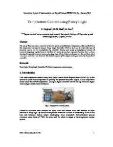
FIG. 1. 共Color online兲 Experimental setup of a cryostat using a GM cryocooler. The inset shows an enlarged view of the sample stage and sample holder for measuring the Seebeck and Nernst coefficients of a single crystal of bismuth.
reinforced-plastic 共FRP兲 dampers to achieve temperature control and stabilization to within a standard deviation of 0.21 mK for a sample temperature of 4.200 0 K. This paper describes the temperature stabilization method employed and its performance. II. EXPERIMENTAL SETUP AND RESULTS
A vacuum cryostat consisting of a two-stage GM cryocooler 共Sumitomo Heavy Industries, SRDK-101D; secondstage capacity of 0.1 W at 4.2 K according to manufacturer’s specifications兲, a feedback temperature controller 共LakeShore, 340兲, and a turbomolecular pumping system was utilized in these experiments. Figure 1 shows a schematic diagram of the cryostat with a superconducting magnet cooled by another cryocooler. All the measurement devices used for acquiring data were connected by IEEE-488 cables and were controlled by a personal computer using a program written using LABVIEW software. A thin gold-plated oxygen-free copper block 共RRR⬇ 100兲 was attached to the GM cryocooler head to determine the center location of the cryostat. The main heater 共50 ⍀; the load current was adjusted by the temperature controller at each temperature兲 was installed in the copper block to control the temperature. Under the copper block, a sample stage was set on a sample holder 共both made of the same class of copper兲, and a small heater 共40 ⍀ at 300 K; its load voltage was adjusted兲 was installed on the sample stage and was connected to the sample by a 0.5-mmthick alumina sheet 共see inset in Fig. 1兲. The resistance of the small heater decreased with decreasing temperature, being much less than 250 m⍀ at 4.2 K. To regulate the heating power at the sample stage, a dummy resistance of 80 ⍀ was serially connected at atmospheric pressure. Two calibrated Cernox temperature sensors were attached to the copper
block and onto the sample stage, and their temperatures were automatically controlled via the two pairs of heaters and thermosensors connected to the temperature controller. This setup and equipment have been widely used in lowtemperature and cryogenic systems.5,6 The GM cryocooler cooled the sample from room temperature to a low temperature. Figure 2 shows a time series of the temperature of the copper block after a temperature of 4 K had been achieved when the main and small heaters were switched off. It took about 1 h to reach the minimum temperature of nearly 3.1 K, and fluctuations were approximately 200 mK during this time. This is typical behavior for the temperature of a sample cooled by a GM cryocooler. To reduce the temperature fluctuations, a FRP G10 damper 共thickness: 0.5 or 1.0 mm, diameter: 45 mm; the same diameter as the GM cryocooler head兲 was inserted between the copper block and the GM cryocooler head, and a low-temperature grease was applied to ensure thermal contact. Both were attached by screwing six stainless-steel
FIG. 2. 共Color online兲 Time series of the temperature of a copper block attached to a GM cryocooler without using a heater; 0.5- and 1.0-mm-thick FRP dampers inserted between the GM cooler head and the copper block 共see Fig. 1兲.
094901-3
Hasegawa et al.
FIG. 3. 共Color online兲 Time series of the sample stage temperature using 4.200 0 K temperature feedback with the heater for no FRP damper, 0.76and 0.96-mm-thick FRP dampers between the sample stage and the sample holder, with a 0.5-mm-thick FRP damper inserted between the GM cooler head and the copper block. The temperature of the copper block was controlled to be 3.800 0 K.
screws into screw holes in the head. Figure 2 also shows the time series of the temperature of the copper block with a FRP damper installed. Minimum temperatures of about 3.3 and 3.6 K were achieved using 0.5- and 1.0-mm-thick FRP dampers, respectively. FRP is well known as a thermal isolator for cryogenics. It has not been inserted directly into the heat route from the sample to the GM cryocooler head because many researchers thought it would greatly reduce the refrigeration capacity. In fact, the minimum temperature increased with increasing thickness of the FRP damper. The time required to attain the minimum temperature was over 3 h for a 1.0-mm-thick FRP. In contrast, the time required to attain the minimum temperature for a 0.5-mm-thick FRP was almost identical to that when no FRP damper was used, and the temperature fluctuation was much smaller than that when no FRP damper was present. The measurement results show that the FRP damper reduced the temperature fluctuations. Experiments were performed when the main heater was operated at 3.8 K with no FRP damper, at 3.8 K with a 0.5mm-thick FRP damper, and at 3.95 K with a 1.0-mm-thick FRP damper. The temperature fluctuations of the copper block without a FRP damper were within ⫾200 mK, even when temperature feedback using the heater was applied; this fluctuation is almost identical to when there was no temperature feedback. We conjecture that when the GM cryocooler was operated at temperatures near 4.2 K, the temperature varied too rapidly to stabilize it using the heater even when the proportional–integral–derivative 共PID兲 values of the feedback system were adjusted. On the other hand, the fluctuation when an FRP damper was installed was small, being less than 5 mK. This demonstrates that using an FRP damper can reduce the temperature fluctuations. To obtain more precise temperature control at the sample stage for the sample, a 0.5-mm-thick FRP damper was inserted between the copper block and the GM cryocooler head, and the temperature of the copper block was controlled to be 3.800 0 K. The thermosensor coupled to the sample stage was attached to 0.2-mm-thick copper electrodes on an alumina sheet 共see inset in Fig. 1兲. A small heater was used to control the temperature to be 4.200 0 K. Figure 3 shows a time series of the sample stage temperature when it was con-
Rev. Sci. Instrum. 81, 094901 共2010兲
FIG. 4. 共Color online兲 Normalized frequency distribution of setting 4.200 0 K with no FRP damper and with a 0.76- and 0.96-mm-thick FRP damper between the sample stage and the sample holder based on the data shown in Fig. 3. Dotted lines indicate the calculated normal distributions.
trolled using the heaters and the thermosensors by a PID feedback control temperature controller 共LakeShore, 340兲. The temperature fluctuations of the sample stage were typically within ⫾3 mK when no FRP damper was present; the temperature fluctuated very slowly in a nonperiodic manner. The fluctuation is too large for our estimated requirement of less than 1 mK for measuring the Seebeck and Nernst coefficients at 4.2 K. Therefore, we inserted another FRP G10 damper with a thickness of 0.76 or 0.96 mm 共area: 27 ⫻ 30 mm2兲 between the sample stage and the copper base 共see inset in Fig. 1兲. A low-temperature grease was applied to ensure thermal contact and the damper was fixed by a stainless-steel screw. Figure 3 also shows the time series of the sample stage temperature with this additional FRP damper inserted. When the 0.76- and 0.96-mm-thick FRP dampers were inserted, temperature fluctuations with ⫾0.5 and ⫾1 mK were achieved, respectively. We were unable to stabilize the temperature by increasing the thickness of the FRP damper due to its high thermal resistance; therefore, this FRP damper should be thin. The temperature fluctuation results satisfied our estimated requirement of less than 1 mK. Using two FRP dampers in a conventional cryosystem and a temperature feedback system makes it possible to obtain precise temperature control and stabilization even for temperatures as low as 4.2 K. Figure 4 shows the frequency distributions of the results in Fig. 3. If precise temperature control was achieved, a normal distribution should be observed centered on 4.200 0 K, the target temperature. When there was no FRP damper between the sample stage and the copper base, temperature control appears to have been achieved; however, the mode was 4.200 5 K when a normal distribution was fitted to the data and the distribution shape is skewed. In contrast, when two FRP dampers were installed, the modes were exactly 4.200 0 K and these exhibited a normal distribution. Normal distributions were fitted to the data in Fig. 4 and the standard deviation 共兲 was estimated to be 1.16 mK when no FRP damper was installed, 0.21 mK when a 0.78-mm-thick FRP damper was used, and 0.35 mK when a 0.96-mm-thick FRP thick damper was used. These values were obtained when the PID value for the temperature feedback was not completely controlled and the resolution was nearly 0.1 mK due to limitations of the temperature controller. Despite this, the tem-
094901-4
Rev. Sci. Instrum. 81, 094901 共2010兲
Hasegawa et al.
perature fluctuation was much less than that when no FRP damper was inserted 共typically 200 mK兲 and the standard deviation was 0.21 mK using the GM cryocooler. It should be possible to further reduce the standard deviation by optimizing the thicknesses of the two FRP dampers. III. DISCUSSION
The results presented above reveal that the mode of the temperature distribution deviates from the target temperature if heat flow is not controlled by using FRP dampers, whereas it is possible to control the temperature precisely at 4.200 0 K by using FRP dampers in combination with temperature control feedback. In this paper, we focus on temperature control and stabilization at 4.200 0 K; however, excellent temperature regulation over the range of 4.2–300 K can be also achieved with the FRP dampers in place. The standard deviation of the temperature fluctuations in the temperature range of 4.2–300 K was also investigated; it was found to be less than 1.15 mK even at 300 K. Of course, temperature control and stabilization near room temperature are considerably more difficult than at low temperatures due to the lower thermal conductivities of the materials 共e.g., copper兲 used to construct the GM cryocooler. However, the thermal resistance of the FRP damper does not affect the cooling power of the GM cryocooler greatly due to its thinness. The advantages of the described method are that it is very easy to install in a conventional cryosystem, it is very inexpensive compared to the cost of a GM cryocooler, and it has no running costs. Moreover, unlike cryosystems that use liquid helium, general cryocoolers operate independently of the position in which they are installed. Thus, the temperature can be controlled in any location. Although the minimum achievable temperature was increased from 3.2 K without a FRP damper to 3.3 K with a FRP damper 共see Fig. 2兲, this difference is relatively small. In addition, a longer cooling time is required. For example, cooling from 300 to 4.0 K took 5 h with no FRP damper, whereas it took about 6 h when FRP dampers were installed 共the cooling time varies depending on the power of the cryocooler used and the heat capacity of its head兲. However, this cooling time is very reasonable, only requiring an additional 1 h to achieve the minimum temperature from 300 K. Many researchers use slow ramping times to avoid damaging the samples when changing the temperature. Based on these considerations, we conclude that there are no major disadvantages associated with the described
method and that using FRP dampers to stabilize and control the temperature makes it possible to use cryosystems based on a GM cryocooler. ACKNOWLEDGMENTS
This research was supported in part by a Grant-in-Aid for the Encouragement of Young Scientists from the Japan Society for the Promotion of Science, the Science and Technology Foundation of Japan, the Murata Science Foundation, the Sumitomo Foundation, the Research Foundation for Material Science, and the Asahi Glass Foundation. This work was performed under the auspices of the National Institute for Fusion Science 共NIFS兲 Collaborative Research 共Grant No. NIFS08KYBI007兲 and NINS’s Creating Innovative Research Fields Project 共Grant No. NINS08KEIN0091兲. The authors are grateful to Dr. Akira Endo of University of Tokyo for valuable suggestions. H. O. McMahon and W. E. Gifford, Adv. Cryog. Eng. 5, 354 共1960兲. H. O. McMahon, Cryogenics 1, 65 共1960兲. 3 M. Nagao, T. Inaguchi, H. Yoshimura, T. Yamada, and M. Iwamoto, Adv. Cryog. Eng. 35, 1251 共1990兲. 4 M. Nagao, T. Inaguchi, H. Yoshimura, S. Nakamura, T. Yamada, T. Matsumoto, S. Nakagawa, K. Moritsu, and T. Watanage, Adv. Cryog. Eng. 39, 1327 共1994兲. 5 Y. Iwasa, Case Studies in Superconducting Magnets: Design and Operational Issues, 2nd ed. 共Springer, New York, 2009兲. 6 For example, Lakeshore 340 Temperature Controller Manual, http:// www.lakeshore.com/pdf_files/instruments/340_Manual.pdf. 7 Y. Hasegawa, Y. Ishikawa, T. Komine, T. E. Huber, A. Suzuki, H. Morita, and H. Shirai, Appl. Phys. Lett. 85, 917 共2004兲. 8 Y. Hasegawa, Y. Ishikawa, H. Morita, T. Komine, H. Shirai, and H. Nakamura, J. Appl. Phys. 97, 083907 共2005兲. 9 Y. Hasegawa, H. Nakano, H. Morita, A. Kurokouchi, K. Wada, T. Komine, and H. Nakamura, J. Appl. Phys. 101, 033704 共2007兲. 10 Y. Hasegawa, H. Nakano, H. Morita, T. Komine, H. Okumura, and H. Nakamura, J. Appl. Phys. 102, 073701 共2007兲. 11 H. Iwasaki, H. Morita, and Y. Hasegawa, Jpn. J. Appl. Phys. 47, 3576 共2008兲. 12 Y. Hasegawa, H. Morita, T. Komine, T. Taguchi, and S. Nakamura, J. Electron. Mater. 38, 944 共2009兲. 13 Y. Hasegawa, M. Murata, D. Nakamura, T. Komine, T. Taguchi, and S. Nakamura, J. Appl. Phys. 105, 103715 共2009兲. 14 M. Murata, D. Nakamura, Y. Hasegawa, T. Komine, T. Taguchi, S. Nakamura, V. Jovovic, and J. P. Heremans, Appl. Phys. Lett. 94, 192104 共2009兲. 15 M. Murata, D. Nakamura, Y. Hasegawa, T. Komine, T. Taguchi, S. Nakamura, V. Jovovic, C. M. Jawaroski, and J. P. Heremans, J. Appl. Phys. 105, 113706 共2009兲. 16 M. Matsuo, A. Endo, N. Hatano, H. Nakamura, R. Shirasaki, and K. Sugihara, Phys. Rev. B 80, 075313 共2009兲. 17 G. K. White, Experimental Techniques in Low-Temperature Physics, 3rd ed. 共Clarendon, Oxford, 1979兲. 1 2